Page 29 - Elementary_Linear_Algebra_with_Applications_Anton__9_edition

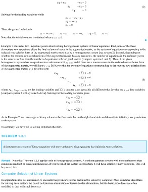
(2)

Solving for the leading variables yields

Thus, the general solution is .
Note that the trivial solution is obtained when

Example 7 illustrates two important points about solving homogeneous systems of linear equations. First, none of the three

elementary row operations alters the final column of zeros in the augmented matrix, so the system of equations corresponding to the

reduced row-echelon form of the augmented matrix must also be a homogeneous system [see system 2]. Second, depending on

whether the reduced row-echelon form of the augmented matrix has any zero rows, the number of equations in the reduced system

is the same as or less than the number of equations in the original system [compare systems 1 and 2]. Thus, if the given

homogeneous system has m equations in n unknowns with , and if there are r nonzero rows in the reduced row-echelon form

of the augmented matrix, we will have . It follows that the system of equations corresponding to the reduced row-echelon form

of the augmented matrix will have the form

(3)

where , , …, are the leading variables and denotes sums (possibly all different) that involve the free variables
[compare system 3 with system 2 above]. Solving for the leading variables gives

As in Example 7, we can assign arbitrary values to the free variables on the right-hand side and thus obtain infinitely many solutions
to the system.
In summary, we have the following important theorem.

THEOREM 1.2.1

A homogeneous system of linear equations with more unknowns than equations has infinitely many solutions.

Remark Note that Theorem 1.2.1 applies only to homogeneous systems. A nonhomogeneous system with more unknowns than
equations need not be consistent (Exercise 28); however, if the system is consistent, it will have infinitely many solutions. This will
be proved later.

Computer Solution of Linear Systems

In applications it is not uncommon to encounter large linear systems that must be solved by computer. Most computer algorithms
for solving such systems are based on Gaussian elimination or Gauss–Jordan elimination, but the basic procedures are often
modified to deal with such issues as