Page 861 - Elementary_Linear_Algebra_with_Applications_Anton__9_edition

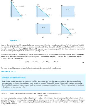
Figure 11.3.1

It can be shown that the feasible region of a linear programming problem has a boundary consisting of a finite number of straight
line segments. If the feasible region can be enclosed in a sufficiently large circle, it is called bounded (Figure 11.3.1e); otherwise,
it is called unbounded (see Figure 11.3.5). If the feasible region is empty (contains no points), then the constraints are inconsistent
and the linear programming problem has no solution (see Figure 11.3.6).

Those boundary points of a feasible region that are intersections of two of the straight line boundary segments are called extreme
points. (They are also called corner points and vertex points.) For example, in Figure 11.3.1e, we see that the feasible region of
Example 1 has four extreme points:

(4)

The importance of the extreme points of a feasible region is shown by the following theorem.
THEOREM 11.3.1

Maximum and Minimum Values
If the feasible region of a linear programming problem is nonempty and bounded, then the objective function attains both a
maximum and a minimum value, and these occur at extreme points of the feasible region. If the feasible region is unbounded,
then the objective function may or may not attain a maximum or minimum value; however, if it attains a maximum or minimum
value, it does so at an extreme point.

Figure 11.3.2 suggests the idea behind the proof of this theorem. Since the objective function

of a linear programming problem is a linear function of and , its level curves (the curves along which z has constant values)
are straight lines. As we move in a direction perpendicular to these level curves, the objective function either increases or decreases
monotonically. Within a bounded feasible region, the maximum and minimum values of z must therefore occur at extreme points,
as Figure 11.3.2 indicates.