Page 21 - Pra U STPM 2022 Penggal 2 - Mathematics

Mathematics Semester 2 STPM Chapter 4 Differential Equations
A solution of the differential equation that contains an arbitrary constant is known as a general solution.

Example 4

y
2
Show that y = A 1 x – 1 2 is a solution of the differential equation dy = x – 1 . Hence, find the value of A
x + 1
2
dx
2Bhd. All Rights Reserved.
if y = 1 when x = 2.
x – 1
Solution: Given y = A 1 x + 1 2 ...................................
2
dy 2A
Thus, 2y = ......................................
dx (x + 1) 2
From ,
1
A = y 2 x + 1 2
x – 1
Substitute into equation ,
dy 2y 2 x + 1
2y = 2 1 2
dx (x + 1) x – 1
dy y
i.e. =
2
dx x – 1
y
1
Thus, y = A x – 1 2 is a solution of the differential equation dy = x – 1 .
2
2
x + 1
dx
Hence, with the condition y = 1 when x = 2, from equation ,
Penerbitan Pelangi Sdn
1
2
1 = A 2 – 1
2 + 1
A = 3
1
2
Thus, y = 3 x – 1 2 4
x + 1
In Example 4, the value of A can be determined from the given condition.
A general solution that satisfies certain conditions (either initial conditions or boundary conditions) so that
the value of the arbitrary constant in the solution is obtained is
called the particular solution.
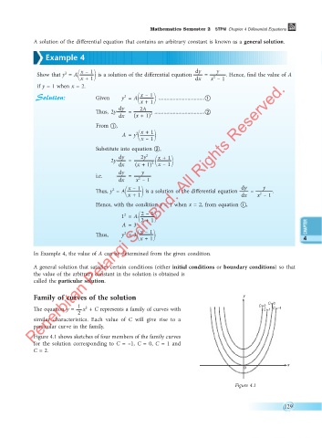
Family of curves of the solution y
C= 0
The equation y = 1 x + C represents a family of curves with C = 2 C= 1 C= –1
2
2
similar characteristics. Each value of C will give rise to a
particular curve in the family.
Figure 4.1 shows sketches of four members of the family curves
for the solution corresponding to C = –1, C = 0, C = 1 and
C = 2.

x
0

Figure 4.1

129

04 STPM Math(T) T2.indd 129 28/01/2022 5:44 PM