Page 132 - Jolliffe I. Principal Component Analysis

5.3. Biplots
101

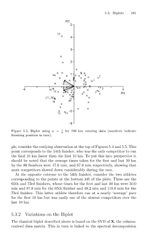
Figure 5.5. Biplot using α = 1 for 100 km running data (numbers indicate
2
finishing position in race).

ple, consider the outlying observation at the top of Figures 5.4 and 5.5. This
point corresponds to the 54th finisher, who was the only competitor to run
the final 10 km faster than the first 10 km. To put this into perspective it
should be noted that the average times taken for the first and last 10 km
by the 80 finishers were 47.6 min, and 67.0 min respectively, showing that
most competitors slowed down considerably during the race.
At the opposite extreme to the 54th finisher, consider the two athletes
corresponding to the points at the bottom left of the plots. These are the
65th and 73rd finishers, whose times for the first and last 10 km were 50.0
min and 87.8 min for the 65th finisher and 48.2 min and 110.0 min for the
73rd finisher. This latter athlete therefore ran at a nearly ‘average’ pace
for the first 10 km but was easily one of the slowest competitors over the
last 10 km.

5.3.2 Variations on the Biplot

The classical biplot described above is based on the SVD of X, the column-
centred data matrix. This in turn is linked to the spectral decomposition