Page 147 - Jolliffe I. Principal Component Analysis

6. Choosing a Subset of Principal Components or Variables
116

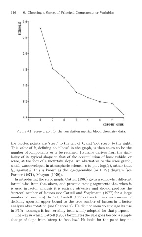
Figure 6.1. Scree graph for the correlation matrix: blood chemistry data.

the plotted points are ‘steep’ to the left of k, and ‘not steep’ to the right.
This value of k, defining an ‘elbow’ in the graph, is then taken to be the
number of components m to be retained. Its name derives from the simi-
larity of its typical shape to that of the accumulation of loose rubble, or
scree, at the foot of a mountain slope. An alternative to the scree graph,
which was developed in atmospheric science, is to plot log(l k ), rather than
l k , against k; this is known as the log-eigenvalue (or LEV) diagram (see
Farmer (1971), Maryon (1979)).
In introducing the scree graph, Cattell (1966) gives a somewhat different
formulation from that above, and presents strong arguments that when it
is used in factor analysis it is entirely objective and should produce the
‘correct’ number of factors (see Cattell and Vogelmann (1977) for a large
number of examples). In fact, Cattell (1966) views the rule as a means of
deciding upon an upper bound to the true number of factors in a factor
analysis after rotation (see Chapter 7). He did not seem to envisage its use
in PCA, although it has certainly been widely adopted for that purpose.
The way in which Cattell (1966) formulates the rule goes beyond a simple
change of slope from ‘steep’ to ‘shallow.’ He looks for the point beyond