Page 152 - Jolliffe I. Principal Component Analysis

121
6.1. How Many Principal Components?
(1982), the number of terms in the estimate for X, corresponding to the
number of PCs, is successively taken as 1, 2,... , and so on, until overall
prediction of the x ij is no longer significantly improved by the addition of
extra terms (PCs). The number of PCs to be retained, m, is then taken to
be the minimum number necessary for adequate prediction.
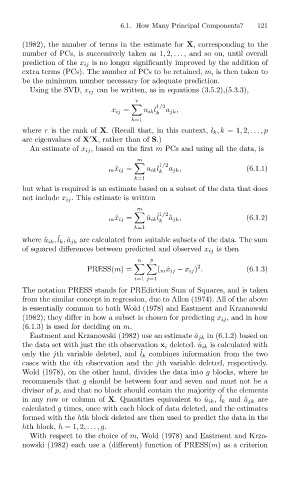
Using the SVD, x ij can be written, as in equations (3.5.2),(5.3.3),
r
1/2
x ij = u ik l a jk ,
k
k=1
where r is the rank of X. (Recall that, in this context, l k ,k =1, 2,... ,p
are eigenvalues of X X, rather than of S.)

An estimate of x ij , based on the first m PCs and using all the data, is
m
1/2
m ˜x ij = u ik l a jk , (6.1.1)
k
k=1
but what is required is an estimate based on a subset of the data that does
not include x ij . This estimate is written
m
1/2
m ˆx ij = ˆ u ik l ˆ ˆ a jk , (6.1.2)
k
k=1
ˆ
where ˆu ik , l k , ˆa jk are calculated from suitable subsets of the data. The sum
of squared differences between predicted and observed x ij is then
n p
2
PRESS(m)= ( m ˆx ij − x ij ) . (6.1.3)
i=1 j=1
The notation PRESS stands for PREdiction Sum of Squares, and is taken
from the similar concept in regression, due to Allen (1974). All of the above
is essentially common to both Wold (1978) and Eastment and Krzanowski
(1982); they differ in how a subset is chosen for predicting x ij , and in how
(6.1.3) is used for deciding on m.
Eastment and Krzanowski (1982) use an estimate ˆa jk in (6.1.2) based on
the data set with just the ith observation x i deleted. ˆu ik is calculated with
ˆ
only the jth variable deleted, and l k combines information from the two
cases with the ith observation and the jth variable deleted, respectively.
Wold (1978), on the other hand, divides the data into g blocks, where he
recommends that g should be between four and seven and must not be a
divisor of p, and that no block should contain the majority of the elements
ˆ
in any row or column of X. Quantities equivalent to ˆu ik , l k and ˆa jk are
calculated g times, once with each block of data deleted, and the estimates
formed with the hth block deleted are then used to predict the data in the
hth block, h =1, 2,... ,g.
With respect to the choice of m, Wold (1978) and Eastment and Krza-
nowski (1982) each use a (different) function of PRESS(m) as a criterion