Page 156 - Jolliffe I. Principal Component Analysis

125
6.1. How Many Principal Components?
needs to be estimated; an obvious estimate is the average of the (p − q)
smallest eigenvalues of S.
Besse and de Falguerolles (1993) start from the same fixed effects model
and concentrate on the special case just noted. They modify the loss
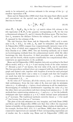
function to become
2

L q = 1 ˆ (6.1.9)
P q − P q ,
2
ˆ
where P q = A q A q , A q is the (p × q) matrix whose kth column is the

ˆ
kth eigenvalue of S, P q is the quantity corresponding to P q for the true
q-dimensional subspace F q ,and . denotes Euclidean norm. The loss func-
tion L q measures the distance between the subspace F q and its estimate
ˆ
F q spanned by the columns of A q .
The risk function that Besse and de Falguerolles (1993) seek to mini-
mize is R q = E[L q ]. As with f q , R q must be estimated, and Besse and
de Falguerolles (1993) compare four computationally intensive ways of do-
ing so, three of which were suggested by Besse (1992), building on ideas
from Daudin et al. (1988, 1989). Two are bootstrap methods; one is based
on bootstrapping residuals from the q-dimensional model, while the other
bootstraps the data themselves. A third procedure uses a jackknife esti-
mate and the fourth, which requires considerably less computational effort,
constructs an approximation to the jackknife.
Besse and de Falguerolles (1993) simulate data sets according to the fixed
effects model, with p = 10, q = 4 and varying levels of the noise variance
2
2
σ . Because q and σ are known, the true value of R q can be calculated.
The four procedures outlined above are compared with the traditional scree
graph and Kaiser’s rule, together with boxplots of scores for each principal
component. In the latter case a value m is sought such that the boxplots
are much less wide for components (m +1), (m +2),...,p than they are
for components 1, 2,... ,m.
2
As the value of σ increases, all of the criteria, new or old, deteriorate in
their performance. Even the true value of R q does not take its minimum
value at q = 4, although q = 4 gives a local minimum in all the simulations.
Bootstrapping of residuals is uninformative regarding the value of q, but
the other three new procedures each have strong local minima at q =4.All
methods have uninteresting minima at q =1 and at q = p, but the jackknife
techniques also have minima at q =6, 7 which become more pronounced
2
as σ increases. The traditional methods correctly choose q = 4 for small
2
2
σ , but become less clear as σ increases.
The plots of the risk estimates are very irregular, and both Besse (1992)
and Besse and de Falguerolles (1993) note that they reflect the important
feature of stability of the subspaces retained. Many studies of stability (see,
for example, Sections 10.2, 10.3, 11.1 and Besse, 1992) show that pairs of
consecutive eigenvectors are unstable if their corresponding eigenvalues are
of similar size. In a similar way, Besse and de Falguerolles’ (1993) risk