Page 394 - Jolliffe I. Principal Component Analysis

13.5. Common Principal Components
359
values of p, q and sample size in his tables closest to those of the present
example. Hence, if Krzanowski’s tables are at all relevant for correlation
matrices, the sets of the first three PCs are not significantly different for
the three years 1982, 1983, 1984 as might be expected from such small
angles.
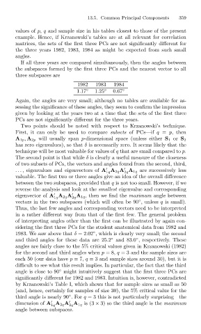
If all three years are compared simultaneously, then the angles between
the subspaces formed by the first three PCs and the nearest vector to all
three subspaces are
1982 1983 1984
1.17 ◦ 1.25 ◦ 0.67 ◦
Again, the angles are very small; although no tables are available for as-
sessing the significance of these angles, they seem to confirm the impression
given by looking at the years two at a time that the sets of the first three
PCs are not significantly different for the three years.
Two points should be noted with respect to Krzanowski’s technique.
First, it can only be used to compare subsets of PCs—if q = p, then
A 1p , A 2p will usually span p-dimensional space (unless either S 1 or S 2
has zero eigenvalues), so that δ is necessarily zero. It seems likely that the
technique will be most valuable for values of q that are small compared to p.
The second point is that while δ is clearly a useful measure of the closeness
of two subsets of PCs, the vectors and angles found from the second, third,
..., eigenvalues and eigenvectors of A A 2q A A 1q are successively less

1q 2q
valuable. The first two or three angles give an idea of the overall difference
between the two subspaces, provided that q is not too small. However, if we
reverse the analysis and look at the smallest eigenvalue and corresponding
eigenvector of A A 2q A A 1q , then we find the maximum angle between

1q 2q
◦
vectors in the two subspaces (which will often be 90 , unless q is small).
Thus, the last few angles and corresponding vectors need to be interpreted
in a rather different way from that of the first few. The general problem
of interpreting angles other than the first can be illustrated by again con-
sidering the first three PCs for the student anatomical data from 1982 and
1983. We saw above that δ =2.02 , which is clearly very small; the second
◦
◦
◦
and third angles for these data are 25.2 and 83.0 , respectively. These
angles are fairly close to the 5% critical values given in Krzanowski (1982)
for the second and third angles when p =8, q = 3 and the sample sizes are
each 50 (our data have p =7, q = 3 and sample sizes around 30), but it is
difficult to see what this result implies. In particular, the fact that the third
angle is close to 90 might intuitively suggest that the first three PCs are
◦
significantly different for 1982 and 1983. Intuition is, however, contradicted
by Krzanowski’s Table I, which shows that for sample sizes as small as 50
(and, hence, certainly for samples of size 30), the 5% critical value for the
◦
third angle is nearly 90 .For q = 3 this is not particularly surprising—the

dimension of A A 2q A A 1q is (3 × 3) so the third angle is the maximum
1q 2q
angle between subspaces.