Page 397 - Jolliffe I. Principal Component Analysis

13. Principal Component Analysis for Special Types of Data
362
components which diagonalize the covariance or correlation matrices reflect
the most important sources of variation in the data.’
Muller (1982) suggests that canonical correlation analysis of PCs (see
Section 9.3) provides a way of comparing the PCs based on two sets of
variables, and cites some earlier references. When the two sets of variables
are, in fact, the same variables measured for two groups of observations,
Muller’s analysis is equivalent to that of Krzanowski (1979b); the latter
paper notes the links between canonical correlation analysis and its own
technique.
In a series of five technical reports, Preisendorfer and Mobley (1982) ex-
amine various ways of comparing data sets measured on the same variables
at different times, and part of their work involves comparison of PCs from
different sets (see, in particular, their third report, which concentrates on
comparing the singular value decompositions (SVDs, Section 3.5) of two
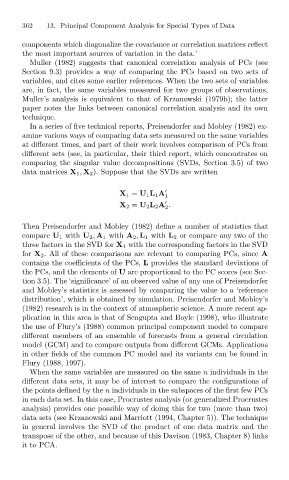
data matrices X 1 , X 2 ). Suppose that the SVDs are written

X 1 = U 1 L 1 A 1

X 2 = U 2 L 2 A .
2
Then Preisendorfer and Mobley (1982) define a number of statistics that
compare U 1 with U 2 , A 1 with A 2 , L 1 with L 2 or compare any two of the
three factors in the SVD for X 1 with the corresponding factors in the SVD
for X 2 . All of these comparisons are relevant to comparing PCs, since A
contains the coefficients of the PCs, L provides the standard deviations of
the PCs, and the elements of U are proportional to the PC scores (see Sec-
tion 3.5). The ‘significance’ of an observed value of any one of Preisendorfer
and Mobley’s statistics is assessed by comparing the value to a ‘reference
distribution’, which is obtained by simulation. Preisendorfer and Mobley’s
(1982) research is in the context of atmospheric science. A more recent ap-
plication in this area is that of Sengupta and Boyle (1998), who illustrate
the use of Flury’s (1988) common principal component model to compare
different members of an ensemble of forecasts from a general circulation
model (GCM) and to compare outputs from different GCMs. Applications
in other fields of the common PC model and its variants can be found in
Flury (1988, 1997).
When the same variables are measured on the same n individuals in the
different data sets, it may be of interest to compare the configurations of
the points defined by the n individuals in the subspaces of the first few PCs
in each data set. In this case, Procrustes analysis (or generalized Procrustes
analysis) provides one possible way of doing this for two (more than two)
data sets (see Krzanowski and Marriott (1994, Chapter 5)). The technique
in general involves the SVD of the product of one data matrix and the
transpose of the other, and because of this Davison (1983, Chapter 8) links
it to PCA.