Page 53 - Jolliffe I. Principal Component Analysis

2. Properties of Population Principal Components
22
A major argument for using correlation—rather than covariance—
matrices to define PCs is that the results of analyses for different sets
of random variables are more directly comparable than for analyses based
on covariance matrices. The big drawback of PCA based on covariance ma-
trices is the sensitivity of the PCs to the units of measurement used for
each element of x. If there are large differences between the variances of the
elements of x, then those variables whose variances are largest will tend
to dominate the first few PCs (see, for example, Section 3.3). This may
be entirely appropriate if all the elements of x are measured in the same
units, for example, if all elements of x are anatomical measurements on a
particular species of animal, all recorded in centimetres, say. Even in such
examples, arguments can be presented for the use of correlation matrices
(see Section 4.1). In practice, it often occurs that different elements of x are
completely different types of measurement. Some might be lengths, some
weights, some temperatures, some arbitrary scores on a five-point scale,
and so on. In such a case, the structure of the PCs will depend on the
choice of units of measurement, as is illustrated by the following artificial
example.
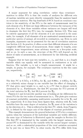
Suppose that we have just two variables, x 1 , x 2 , and that x 1 is a length
variable which can equally well be measured in centimetres or in mil-
limetres. The variable x 2 is not a length measurement—it might be a
weight, in grams, for example. The covariance matrices in the two cases
are, respectively,

80 44 8000 440
Σ 1 = and Σ 2 = .
44 80 440 80
ThefirstPCis0.707x 1 +0.707x 2 for Σ 1 and 0.998x 1 +0.055x 2 for Σ 2 ,
so a relatively minor change in one variable has the effect of changing a
PC that gives equal weight to x 1 and x 2 to a PC that is almost entirely
dominated by x 1 . Furthermore, the first PC accounts for 77.5 percent of
the total variation for Σ 1 , but 99.3 percent for Σ 2 .
Figures 2.1 and 2.2 provide another way of looking at the differences be-
tween PCs for the two scales of measurement in x 1 . The plots give contours
of constant probability, assuming multivariate normality for x for Σ 1 and
Σ 2 , respectively. It is clear from these figures that, whereas with Σ 1 both
variables have the same degree of variation, for Σ 2 most of the variation is
in the direction of x 1 . This is reflected in the first PC, which, from Property
G1, is defined by the major axis of the ellipses of constant probability.
This example demonstrates the general behaviour of PCs for a covariance
matrix when the variances of the individual variables are widely different;
the same type of behaviour is illustrated again for samples in Section 3.3.
The first PC is dominated by the variable with the largest variance, the
second PC is dominated by the variable with the second largest variance,
and so on, with a substantial proportion of the total variation accounted
for by just two or three PCs. In other words, the PCs differ little from