Page 185 - Jolliffe I. Principal Component Analysis

7. Principal Component Analysis and Factor Analysis
154
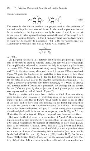
chosen to maximize

m
p

Q = b 4 − 1 p b 2 2
. (7.2.2)
p
jk jk
k=1 j=1 j=1
The terms in the square brackets are proportional to the variances of
squared loadings for each rotated factor. In the usual implementations of
factor analysis the loadings are necessarily between −1 and 1, so the cri-
terion tends to drive squared loadings towards the end of the range 0 to 1,
and hence loadings towards −1, 0 or 1 and away from intermediate values,
as required. The quantity Q in equation (7.2.2) is the raw varimax criterion.
A normalized version is also used in which b jk is replaced by
b jk
2
b
m
k=1 jk
in (7.2.2).
As discussed in Section 11.1, rotation can be applied to principal compo-
nent coefficients in order to simplify them, as is done with factor loadings.
The simplification achieved by rotation can help in interpreting the factors
or rotated PCs. This is illustrated nicely using diagrams (see Figures 7.1
and 7.2) in the simple case where only m = 2 factors or PCs are retained.
Figure 7.1 plots the loadings of ten variables on two factors. In fact, these
loadings are the coefficients a 1 , a 2 for the first two PCs from the exam-
ple presented in detail later in the chapter, normalized so that a a k = l k ,

k
where l k is the kth eigenvalue of S, rather than a a k = 1. When an orthog-

k
onal rotation method (varimax) is performed, the loadings for the rotated
factors (PCs) are given by the projections of each plotted point onto the
axes represented by dashed lines in Figure 7.1.
Similarly, rotation using an oblique rotation method (direct quartimin)
gives loadings after rotation by projecting onto the new axes shown in
Figure 7.2. It is seen that in Figure 7.2 all points lie close to one or other
of the axes, and so have near-zero loadings on the factor represented by
the other axis, giving a very simple structure for the loadings. The loadings
implied for the rotated factors in Figure 7.1, whilst having simpler structure
than the original coefficients, are not as simple as those for Figure 7.2, thus
illustrating the advantage of oblique, compared to orthogonal, rotation.
Returning to the first stage in the estimation of Λ and Ψ, there is some-
times a problem with identifiability, meaning that the size of the data set
is too small compared to the number of parameters to allow those param-
eters to be estimated (Jackson, 1991, Section 17.2.6; Everitt and Dunn,
2001, Section 12.3)). Assuming that identifiability is not a problem, there
are a number of ways of constructing initial estimates (see, for example,
Lewis-Beck (1994, Section II.2); Rencher (1998, Section 10.3); Everitt and
Dunn (2001, Section 12.2)). Some, such as the centroid method (see Cat-
tell, 1978, Section 2.3), were developed before the advent of computers and