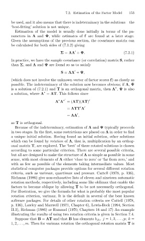
Page 184 - Jolliffe I. Principal Component Analysis

7.2. Estimation of the Factor Model
153
be used, and it also means that there is indeterminacy in the solutions—the
‘best-fitting’ solution is not unique.
Estimation of the model is usually done initially in terms of the pa-
rameters in Λ and Ψ, while estimates of f are found at a later stage.
Given the assumptions of the previous section, the covariance matrix can
be calculated for both sides of (7.1.2) giving

Σ = ΛΛ + Ψ. (7.2.1)
In practice, we have the sample covariance (or correlation) matrix S, rather
than Σ,and Λ and Ψ are found so as to satisfy

S = ΛΛ + Ψ,
(which does not involve the unknown vector of factor scores f) as closely as
possible. The indeterminacy of the solution now becomes obvious; if Λ, Ψ
is a solution of (7.2.1) and T is an orthogonal matrix, then Λ , Ψ is also
∗
∗
a solution, where Λ = ΛT. This follows since

∗
Λ Λ ∗ =(ΛT)(ΛT)

= ΛTT Λ

= ΛΛ ,
as T is orthogonal.
Because of the indeterminacy, estimation of Λ and Ψ typically proceeds
in two stages. In the first, some restrictions are placed on Λ in order to find
a unique initial solution. Having found an initial solution, other solutions
which can be found by rotation of Λ, that is, multiplication by an orthog-
onal matrix T, are explored. The ‘best’ of these rotated solutions is chosen
according to some particular criterion. There are several possible criteria,
but all are designed to make the structure of Λ as simple as possible in some
sense, with most elements of Λ either ‘close to zero’ or ‘far from zero,’ and
with as few as possible of the elements taking intermediate values. Most
statistical computer packages provide options for several different rotation
criteria, such as varimax, quartimax and promax. Cattell (1978, p. 136),
Richman (1986) give non-exhaustive lists of eleven and nineteen automatic
rotation methods, respectively, including some like oblimax that enable the
factors to become oblique by allowing T to be not necessarily orthogonal.
For illustration, we give the formula for what is probably the most popular
rotation criterion, varimax. It is the default in several of the best known
software packages. For details of other rotation criteria see Cattell (1978,
p. 136), Lawley and Maxwell (1971, Chapter 6), Lewis-Beck (1994, Section
II.3), Richman (1986) or Rummel (1970, Chapters 16 and 17) An example
illustrating the results of using two rotation criteria is given in Section 7.4.
Suppose that B = ΛT and that B has elements b jk ,j =1, 2,... ,p; k =
1, 2,... ,m. Then for varimax rotation the orthogonal rotation matrix T is