Page 182 - Jolliffe I. Principal Component Analysis

151
7.1. Models for Factor Analysis
may be estimated and how PCs are, but should perhaps not be, used in
this estimation process. Section 7.3 contains further discussion of differences
and similarities between PCA and factor analysis, and Section 7.4 gives a
numerical example, which compares the results of PCA and factor analysis.
Finally, in Section 7.5, a few concluding remarks are made regarding the
‘relative merits’ of PCA and factor analysis, and the possible use of rotation
with PCA. The latter is discussed further in Chapter 11.
7.1 Models for Factor Analysis

The basic idea underlying factor analysis is that p observed random vari-
ables, x, can be expressed, except for an error term, as linear functions
of m (<p) hypothetical (random) variables or common factors, that
is if x 1 ,x 2 ,...,x p are the variables and f 1 ,f 2 ,...,f m are the factors,
then
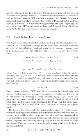
(7.1.1)
x 1 = λ 11 f 1 + λ 12 f 2 + ... + λ 1m f m + e 1
x 2 = λ 21 f 1 + λ 22 f 2 + ... + λ 2m f m + e 2
.
.
.
x p = λ p1 f 1 + λ p2 f 2 + ... + λ pm f m + e p
where λ jk ,j =1, 2,... ,p; k =1, 2,... ,m are constants called the factor
loadings,and e j ,j =1, 2,...,p are error terms, sometimes called specific
factors (because e j is ‘specific’ to x j , whereas the f k are ‘common’ to sev-
eral x j ). Equation (7.1.1) can be rewritten in matrix form, with obvious
notation, as

x = Λf + e. (7.1.2)
One contrast between PCA and factor analysis is immediately ap-
parent. Factor analysis attempts to achieve a reduction from p to
m dimensions by invoking a model relating x 1 ,x 2 ,...,x p to m hy-
pothetical or latent variables. We have seen in Sections 3.9, 5.3 and
6.1.5 that models have been postulated for PCA, but for most prac-
tical purposes PCA differs from factor analysis in having no explicit
model.
The form of the basic model for factor analysis given in (7.1.2) is fairly
standard, although some authors give somewhat different versions. For ex-
ample, there could be three terms on the right-hand side corresponding
to contributions from common factors, specific factors and measurement
errors (Reyment and J¨oreskog, 1993, p. 36), or the model could be made
non-linear. There are a number of assumptions associated with the factor
model, as follows:
(i) E[e]= 0, E[f]= 0, E[x]= 0.