Page 33 - Jolliffe I. Principal Component Analysis

1. Introduction
2

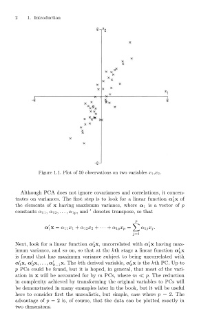
Figure 1.1. Plot of 50 observations on two variables x 1,x 2.

Although PCA does not ignore covariances and correlations, it concen-
trates on variances. The first step is to look for a linear function α x of

1
the elements of x having maximum variance, where α 1 is a vector of p
constants α 11 , α 12 ,...,α 1p ,and denotes transpose, so that

p

α x = α 11 x 1 + α 12 x 2 + ··· + α 1p x p = α 1j x j .
1
j=1

Next, look for a linear function α x, uncorrelated with α x having max-

2
1
imum variance, and so on, so that at the kth stage a linear function α x

k
is found that has maximum variance subject to being uncorrelated with
α x, α x,..., α k−1 x.The kth derived variable, α x is the kth PC. Up to

1
2
k
p PCs could be found, but it is hoped, in general, that most of the vari-
ation in x will be accounted for by m PCs, where m p. The reduction
in complexity achieved by transforming the original variables to PCs will
be demonstrated in many examples later in the book, but it will be useful
here to consider first the unrealistic, but simple, case where p =2.The
advantage of p = 2 is, of course, that the data can be plotted exactly in
two dimensions.