Page 35 - Jolliffe I. Principal Component Analysis

1. Introduction
4

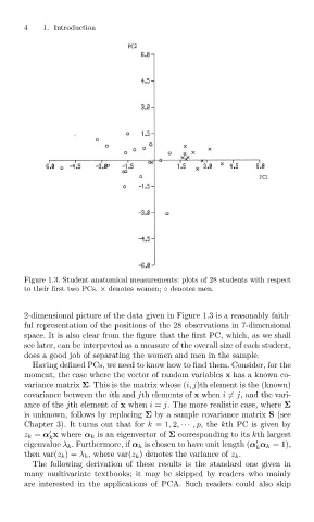
Figure 1.3. Student anatomical measurements: plots of 28 students with respect
to their first two PCs. × denotes women; ◦ denotes men.

2-dimensional picture of the data given in Figure 1.3 is a reasonably faith-
ful representation of the positions of the 28 observations in 7-dimensional
space. It is also clear from the figure that the first PC, which, as we shall
see later, can be interpreted as a measure of the overall size of each student,
does a good job of separating the women and men in the sample.
Having defined PCs, we need to know how to find them. Consider, for the
moment, the case where the vector of random variables x has a known co-
variance matrix Σ. This is the matrix whose (i, j)th element is the (known)
covariance between the ith and jth elements of x when i = j, and the vari-
ance of the jth element of x when i = j. The more realistic case, where Σ
is unknown, follows by replacing Σ by a sample covariance matrix S (see
Chapter 3). It turns out that for k =1, 2, ··· ,p,the kth PC is given by
z k = α x where α k is an eigenvector of Σ corresponding to its kth largest

k
eigenvalue λ k . Furthermore, if α k is chosen to have unit length (α α k = 1),

k
then var(z k )= λ k , where var(z k ) denotes the variance of z k .
The following derivation of these results is the standard one given in
many multivariate textbooks; it may be skipped by readers who mainly
are interested in the applications of PCA. Such readers could also skip