Page 34 - Jolliffe I. Principal Component Analysis

1.1. Definition and Derivation of Principal Components

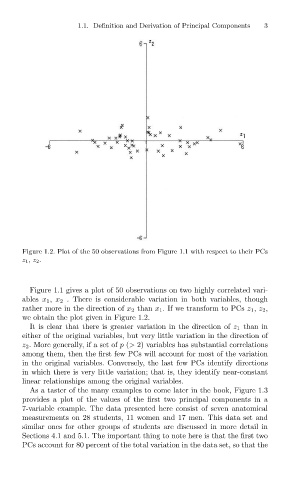
Figure 1.2. Plot of the 50 observations from Figure 1.1 with respect to their PCs 3
z 1, z 2.

Figure 1.1 gives a plot of 50 observations on two highly correlated vari-
ables x 1 , x 2 . There is considerable variation in both variables, though
rather more in the direction of x 2 than x 1 . If we transform to PCs z 1 , z 2 ,
we obtain the plot given in Figure 1.2.
It is clear that there is greater variation in the direction of z 1 than in
either of the original variables, but very little variation in the direction of
z 2 . More generally, if a set of p (> 2) variables has substantial correlations
among them, then the first few PCs will account for most of the variation
in the original variables. Conversely, the last few PCs identify directions
in which there is very little variation; that is, they identify near-constant
linear relationships among the original variables.
As a taster of the many examples to come later in the book, Figure 1.3
provides a plot of the values of the first two principal components in a
7-variable example. The data presented here consist of seven anatomical
measurements on 28 students, 11 women and 17 men. This data set and
similar ones for other groups of students are discussed in more detail in
Sections 4.1 and 5.1. The important thing to note here is that the first two
PCs account for 80 percent of the total variation in the data set, so that the