Page 388 - Applied Statistics with R

388 CHAPTER 16. VARIABLE SELECTION AND MODEL BUILDING

We can see that the solid blue curve models this data rather nicely. The dashed
orange curve fits the points better, making smaller errors, however it is unlikely
that it is correctly modeling the true relationship between and . It is fitting
the random noise. This is an example of overfitting.
We see that the larger model indeed has a lower RMSE.

sqrt(mean(resid(fit_quad) ^ 2))

## [1] 17.61812

sqrt(mean(resid(fit_big) ^ 2))

## [1] 10.4197

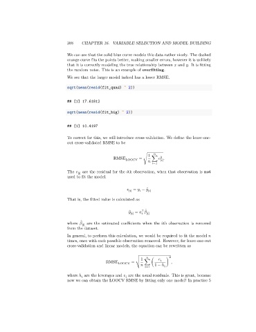
To correct for this, we will introduce cross-validation. We define the leave-one-
out cross-validated RMSE to be

1
2
RMSE LOOCV = √ ∑ .
[ ]
=1
The [ ] are the residual for the th observation, when that observation is not
used to fit the model.

[ ] = − ̂ [ ]

That is, the fitted value is calculated as

⊤ ̂
̂
[ ] = [ ]

̂
where [ ] are the estimated coefficients when the th observation is removed
from the dataset.
In general, to perform this calculation, we would be required to fit the model
times, once with each possible observation removed. However, for leave-one-out
cross-validation and linear models, the equation can be rewritten as

√ 2
√ 1
√
RMSE LOOCV = ∑ ( ) ,
⎷ =1 1 − ℎ
where ℎ are the leverages and are the usual residuals. This is great, because

now we can obtain the LOOCV RMSE by fitting only one model! In practice 5