Page 499 - Elementary_Linear_Algebra_with_Applications_Anton__9_edition

(1)

But , being a difference of vectors in W, is in W; and is orthogonal to W, so the

two terms on the right side of 1 are orthogonal. Thus, by the Theorem of Pythagoras (Theorem

6.2.4),

If , then the second term in this sum will be positive, so

or, equivalently,

Applications of this theorem will be given later in the text.

Least Squares Solutions of Linear Systems

Up to now we have been concerned primarily with consistent systems of linear equations. However, inconsistent linear

systems are also important in physical applications. It is a common situation that some physical problem leads to a linear

system that should be consistent on theoretical grounds but fails to be so because “measurement errors” in the entries

of A and b perturb the system enough to cause inconsistency. In such situations one looks for a value of x that comes “as

close as possible” to being a solution in the sense that it minimizes the value of with respect to the Euclidean inner

product. The quantity can be viewed as a measure of the “error” that results from regarding x as an approximate

solution of the linear system . If the system is consistent and x is an exact solution, then the error is zero, since

. In general, the larger the value of , the more poorly x serves as an approximate solution of the

system.

Least Squares Problem Given a linear system of m equations in n unknowns, find a vector x, if possible, that

minimizes with respect to the Euclidean inner product on . Such a vector is called a least squares solution of

.

Remark To understand the origin of the term least squares, let , which we can view as the error vector that

results from the approximation x. If , then a least squares solution minimizes

; hence it also minimizes . Hence the term least squares.

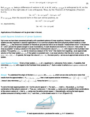
To solve the least squares problem, let W be the column space of A. For each matrix x, the product is a linear
combination of the column vectors of A. Thus, as x varies over , the vector varies over all possible linear combinations
of the column vectors of A; that is, varies over the entire column space W. Geometrically, solving the least squares
problem amounts to finding a vector x in such that is the closest vector in W to b (Figure 6.4.2).

Figure 6.4.2
A least squares solution x produces the vector in W closest to b.