Page 164 - Jolliffe I. Principal Component Analysis

6.2. Choosing m, the Number of Components: Examples
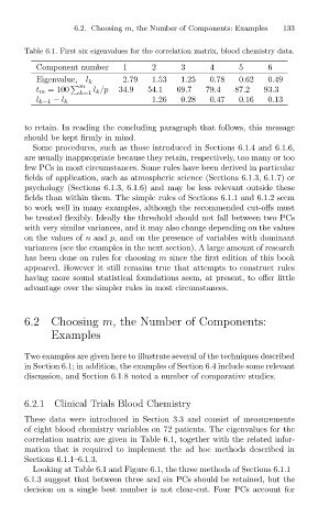
Table 6.1. First six eigenvalues for the correlation matrix, blood chemistry data.
1
Component number
0.62
0.49
0.78
2.79 2 3 4 5 6 133
1.53
1.25
Eigenvalue, l k

t m = 100 k=1 k /p 34.9 54.1 69.7 79.4 87.2 93.3
l
m
1.26 0.28 0.47 0.16 0.13
l k−1 − l k
to retain. In reading the concluding paragraph that follows, this message
should be kept firmly in mind.
Some procedures, such as those introduced in Sections 6.1.4 and 6.1.6,
are usually inappropriate because they retain, respectively, too many or too
few PCs in most circumstances. Some rules have been derived in particular
fields of application, such as atmospheric science (Sections 6.1.3, 6.1.7) or
psychology (Sections 6.1.3, 6.1.6) and may be less relevant outside these
fields than within them. The simple rules of Sections 6.1.1 and 6.1.2 seem
to work well in many examples, although the recommended cut-offs must
be treated flexibly. Ideally the threshold should not fall between two PCs
with very similar variances, and it may also change depending on the values
on the values of n and p, and on the presence of variables with dominant
variances (see the examples in the next section). A large amount of research
has been done on rules for choosing m since the first edition of this book
appeared. However it still remains true that attempts to construct rules
having more sound statistical foundations seem, at present, to offer little
advantage over the simpler rules in most circumstances.

6.2 Choosing m, the Number of Components:
Examples

Two examples are given here to illustrate several of the techniques described
in Section 6.1; in addition, the examples of Section 6.4 include some relevant
discussion, and Section 6.1.8 noted a number of comparative studies.

6.2.1 Clinical Trials Blood Chemistry
These data were introduced in Section 3.3 and consist of measurements
of eight blood chemistry variables on 72 patients. The eigenvalues for the
correlation matrix are given in Table 6.1, together with the related infor-
mation that is required to implement the ad hoc methods described in
Sections 6.1.1–6.1.3.
Looking at Table 6.1 and Figure 6.1, the three methods of Sections 6.1.1–
6.1.3 suggest that between three and six PCs should be retained, but the
decision on a single best number is not clear-cut. Four PCs account for