Page 165 - Jolliffe I. Principal Component Analysis

6. Choosing a Subset of Principal Components or Variables
134
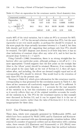
Table 6.2. First six eigenvalues for the covariance matrix, blood chemistry data.
1
2
Component number
Eigenvalue, l k 1704.68 15.07 3 6.98 4 2.64 5 0.13 6 0.07
l k/l ¯ 7.88 0.07 0.03 0.01 0.0006 0.0003
m
l k
k=1
p
t m = 100 98.6 99.4 99.8 99.99 99.995 99.9994
l k
k=1
l k−1 − l k 1689.61 8.09 4.34 2.51 0.06
nearly 80% of the total variation, but it takes six PCs to account for 90%.
A cut-off at l =0.7 for the second criterion retains four PCs, but the next
∗
eigenvalue is not very much smaller, so perhaps five should be retained. In
the scree graph the slope actually increases between k = 3 and 4, but then
falls sharply and levels off, suggesting that perhaps only four PCs should
be retained. The LEV diagram (not shown) is of little help here; it has no
clear indication of constant slope after any value of k, and in fact has its
steepest slope between k =7 and 8.
Using Cattell’s (1966) formulation, there is no strong straight-line be-
haviour after any particular point, although perhaps a cut-off at k =4 is
most appropriate. Cattell suggests that the first point on the straight line
(that is, the ‘elbow’ point) should be retained. However, if we consider the
scree graph in the same light as the test of Section 6.1.4, then all eigen-
values after, and including, the elbow are deemed roughly equal and so all
corresponding PCs should be deleted. This would lead to the retention of
only three PCs in the present case.
Turning to Table 6.2, which gives information for the covariance matrix,
corresponding to that presented for the correlation matrix in Table 6.1, the
three ad hoc measures all conclusively suggest that one PC is sufficient. It
is undoubtedly true that choosing m = 1 accounts for the vast majority
of the variation in x, but this conclusion is not particularly informative
as it merely reflects that one of the original variables accounts for nearly
all the variation in x. The PCs for the covariance matrix in this example
were discussed in Section 3.3, and it can be argued that it is the use of
the covariance matrix, rather than the rules of Sections 6.1.1–6.1.3, that is
inappropriate for these data.

6.2.2 Gas Chromatography Data

These data, which were originally presented by McReynolds (1970), and
which have been analysed by Wold (1978) and by Eastment and Krzanow-
ski (1982), are concerned with gas chromatography retention indices. After
removal of a number of apparent outliers and an observation with a missing
value, there remain 212 (Eastment and Krzanowski) or 213 (Wold) mea-
surements on ten variables. Wold (1978) claims that his method indicates