Page 167 - Jolliffe I. Principal Component Analysis

6. Choosing a Subset of Principal Components or Variables
136

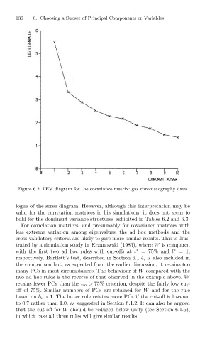
Figure 6.2. LEV diagram for the covariance matrix: gas chromatography data.

logue of the scree diagram. However, although this interpretation may be
valid for the correlation matrices in his simulations, it does not seem to
hold for the dominant variance structures exhibited in Tables 6.2 and 6.3.
For correlation matrices, and presumably for covariance matrices with
less extreme variation among eigenvalues, the ad hoc methods and the
cross-validatory criteria are likely to give more similar results. This is illus-
trated by a simulation study in Krzanowski (1983), where W is compared
∗
∗
with the first two ad hoc rules with cut-offs at t = 75% and l =1,
respectively. Bartlett’s test, described in Section 6.1.4, is also included in
the comparison but, as expected from the earlier discussion, it retains too
many PCs in most circumstances. The behaviour of W compared with the
two ad hoc rules is the reverse of that observed in the example above. W
retains fewer PCs than the t m > 75% criterion, despite the fairly low cut-
off of 75%. Similar numbers of PCs are retained for W and for the rule
based on l k > 1. The latter rule retains more PCs if the cut-off is lowered
to 0.7 rather than 1.0, as suggested in Section 6.1.2. It can also be argued
that the cut-off for W should be reduced below unity (see Section 6.1.5),
in which case all three rules will give similar results.