Page 166 - Jolliffe I. Principal Component Analysis

6.2. Choosing m, the Number of Components: Examples
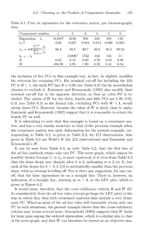
Table 6.3. First six eigenvalues for the covariance matrix, gas chromatography
data.
Component number 1 2 3 4 5 6 135
Eigenvalue, l k 312187 2100 768 336 190 149
l k/l ¯ 9.88 0.067 0.024 0.011 0.006 0.005
m
k=1 l k
t m = 100 p 98.8 99.5 99.7 99.8 99.9 99.94
l k
k=1
l k−1 − l k 310087 1332 432 146 51
R 0.02 0.43 0.60 0.70 0.83 0.99
W 494.98 4.95 1.90 0.92 0.41 0.54
the inclusion of five PCs in this example but, in fact, he slightly modifies
his criterion for retaining PCs. His nominal cut-off for including the kth
PC is R< 1; the sixth PC has R =0.99 (see Table 6.3) but he nevertheless
chooses to exclude it. Eastment and Krzanowski (1982) also modify their
nominal cut-off but in the opposite direction, so that an extra PC is in-
cluded. The values of W for the third, fourth and fifth PCs are 1.90, 0.92,
0.41 (see Table 6.3) so the formal rule, excluding PCs with W< 1, would
retain three PCs. However, because the value of W is fairly close to unity,
Eastment and Krzanowski (1982) suggest that it is reasonable to retain the
fourth PC as well.
It is interesting to note that this example is based on a covariance ma-
trix, and has a very similar structure to that of the previous example when
the covariance matrix was used. Information for the present example, cor-
responding to Table 6.2, is given in Table 6.3, for 212 observations. Also
given in Table 6.3 are Wold’s R (for 213 observations) and Eastment and
Krzanowski’s W.
It can be seen from Table 6.3, as with Table 6.2, that the first two of
the ad hoc methods retain only one PC. The scree graph, which cannot be
sensibly drawn because l 1 l 2 , is more equivocal; it is clear from Table 6.3
that the slope drops very sharply after k = 2, indicating m = 2 (or 1), but
each of the slopes for k =3, 4, 5, 6 is substantially smaller than the previous
slope, with no obvious levelling off. Nor is there any suggestion, for any cut-
off, that the later eigenvalues lie on a straight line. There is, however, an
indication of a straight line, starting at m = 4, in the LEV plot, which is
given in Figure 6.2.
It would seem, therefore, that the cross-validatory criteria R and W dif-
fer considerably from the ad hoc rules (except perhaps the LEV plot) in the
way in which they deal with covariance matrices that include a very domi-
nant PC. Whereas most of the ad hoc rules will invariably retain only one
PC in such situations, the present example shows that the cross-validatory
criteria may retain several more. Krzanowski (1983) suggests that W looks
for large gaps among the ordered eigenvalues, which is a similar aim to that
of the scree graph, and that W can therefore be viewed as an objective ana-