Page 171 - Jolliffe I. Principal Component Analysis

6. Choosing a Subset of Principal Components or Variables
140
one of McCabe’s four criteria when dealing with principal variables.
Of the four criteria, McCabe (1984) argues that only for the first is it
computationally feasible to explore all possible subsets, although the second
can be used to define a stepwise variable-selection procedure; Bhargava and
Ishizuka (1991) describe such a procedure. The third and fourth criteria are
not explored further in McCabe’s paper.
Several of the methods for selecting subsets of variables that preserve
most of the information in the data associate variables with individual PCs.
Cadima and Jolliffe (2001) extend the ideas of Cadima and Jolliffe (1995)
for individual PCs, and look for subsets of variables that best approximate
the subspace spanned by a subset of q PCs, in the the sense that the
subspace spanned by the chosen variables is close to that spanned by the
PCs of interest. A similar comparison of subspaces is the starting point
for Besse and de Falguerolles’s (1993) procedures for choosing the number
of components to retain (see Section 6.1.5). In what follows we restrict
attention to the first q PCs, but the reasoning extends easily to any set of
q PCs.
Cadima and Jolliffe (2001) argue that there are two main ways of assess-
ing the quality of the subspace spanned by a subset of m variables. The
first compares the subspace directly with that spanned by the first q PCs;
the second compares the data with its configuration when projected onto
the m-variable subspaces.
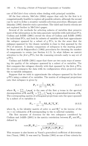
Suppose that we wish to approximate the subspace spanned by the first
q PCs using a subset of m variables. The matrix of orthogonal projections
onto that subspace is given by
1

−
P q = XS X , (6.3.1)
(n − 1) q

l

where S q = k=1 k a k a is the sum of the first q terms in the spectral
q
k
−1
−

decomposition of S,and S = q l a k a is a generalized inverse of S q .
q k=1 k k
The corresponding matrix of orthogonal projections onto the space spanned
by a subset of m variables is
1
I X ,
P m = XI m S −1 (6.3.2)
(n − 1) m m
where I m is the identity matrix of order m and S −1 is the inverse of the
m
(m × m) submatrix of S corresponding to the m selected variables.
The first measure of closeness for the two subspaces considered by
Cadima and Jolliffe (2001) is the matrix correlation between P q and P m ,
defined by
tr(P P m )

. (6.3.3)
q
corr(P q , P m )=
tr(P P q )tr(P P m )

q m
This measure is also known as Yanai’s generalized coefficient of determina-
tion (Yanai, 1980). It was used by Tanaka (1983) as one of four criteria for