Page 418 - Applied Statistics with R

418 CHAPTER 17. LOGISTIC REGRESSION

Now we’ll allow for two modifications of this situation, which will let us use linear
models in many more situations. Instead of using a normal distribution for the
response conditioned on the predictors, we’ll allow for other distributions. Also,
instead of the conditional mean being a linear combination of the predictors, it
can be some function of a linear combination of the predictors.
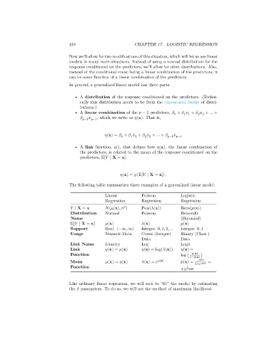
In general, a generalized linear model has three parts:

• A distribution of the response conditioned on the predictors. (Techni-
cally this distribution needs to be from the exponential family of distri-
butions.)
• A linear combination of the − 1 predictors, + + + … +
2 2
1 1
0

−1 −1 , which we write as (x). That is,

(x) = + + + … + −1 −1
2 2
0
1 1
• A link function, (), that defines how (x), the linear combination of
the predictors, is related to the mean of the response conditioned on the
predictors, E[ ∣ X = x].

(x) = (E[ ∣ X = x]) .

The following table summarizes three examples of a generalized linear model:

Linear Poisson Logistic
Regression Regression Regression
2
∣ X = x ( (x), ) Pois( (x)) Bern( (x))
Distribution Normal Poisson Bernoulli
Name (Binomial)
E[ ∣ X = x] (x) (x) (x)
Support Real: (−∞, ∞) Integer: 0, 1, 2, … Integer: 0, 1
Usage Numeric Data Count (Integer) Binary (Class )
Data Data
Link Name Identity Log Logit
Link (x) = (x) (x) = log( (x)) (x) =
Function log ( (x) )
1− (x)
(x)

Mean (x) = (x) (x) = (x) (x) = 1+ (x) =
Function 1
1+ − (x)

Like ordinary linear regression, we will seek to “fit” the model by estimating
the parameters. To do so, we will use the method of maximum likelihood.