Page 423 - Applied Statistics with R

17.2. BINARY RESPONSE 423

sim_logistic_data = function(sample_size = 25, beta_0 = -2, beta_1 = 3) {
x = rnorm(n = sample_size)
eta = beta_0 + beta_1 * x
p = 1 / (1 + exp(-eta))
y = rbinom(n = sample_size, size = 1, prob = p)
data.frame(y, x)
}

You might think, why not simply use ordinary linear regression? Even with a
binary response, our goal is still to model (some function of) E[ ∣ X = x].
However, with a binary response coded as 0 and 1, E[ ∣ X = x] = [ = 1 ∣
X = x] since

E[ ∣ X = x] = 1 ⋅ [ = 1 ∣ X = x] + 0 ⋅ [ = 0 ∣ X = x]
= [ = 1 ∣ X = x]

Then why can’t we just use ordinary linear regression to estimate E[ ∣ X = x],
and thus [ = 1 ∣ X = x]?
To investigate, let’s simulate data from the following model:

(x)
log ( ) = −2 + 3
1 − (x)
Another way to write this, which better matches the function we’re using to
simulate the data:

∣ X = x ∼ Bern( )
i
i

1
= (x ) = 1 + − (x i )

i
(x ) = −2 + 3
i
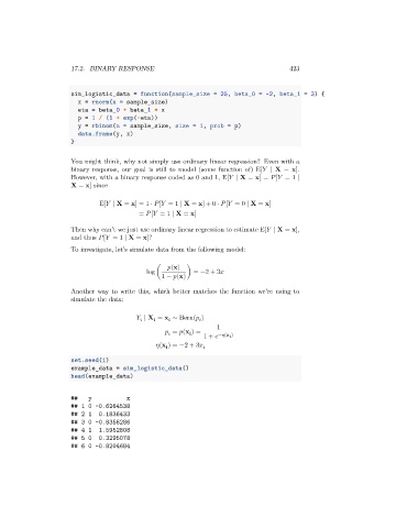
set.seed(1)
example_data = sim_logistic_data()
head(example_data)
## y x
## 1 0 -0.6264538
## 2 1 0.1836433
## 3 0 -0.8356286
## 4 1 1.5952808
## 5 0 0.3295078
## 6 0 -0.8204684