Page 740 - Elementary_Linear_Algebra_with_Applications_Anton__9_edition

9.8 In this section we shall discuss some practical aspects of solving systems of
linear equations, inverting matrices, and finding eigenvalues. Although we have
COMPARISON OF previously discussed methods for performing these computations, we now
PROCEDURES FOR consider their suitability for the computer solution of the large-scale problems
SOLVING LINEAR that arise in real-world applications.
SYSTEMS

Counting Operations

Since computers are limited in the number of decimal places they can carry, they round off or truncate most numerical quantities.
For example, a computer designed to store eight decimal places might record as either .66666667 (rounded off) or .66666666
(truncated).* In either case, an error is introduced that we shall call roundoff error or rounding error.

The main practical considerations in solving linear algebra problems on digital computers are minimizing the computer time (and
thus cost) needed to obtain the solution, and minimizing inaccuracies due to roundoff errors. Thus, a good computer algorithm
uses as few operations and memory accesses as possible, and performs the operations in a way that minimizes the effect of
roundoff errors.

In this text we have studied four methods for solving a linear system, , of n equations in n unknowns:

1. Gaussian elimination with back-substitution

2. Gauss–Jordan elimination

3. Computing , then forming

4. Cramer's rule

To determine how these methods compare as computational tools, we need to know how many arithmetic operations each requires.
It is usual to group divisions and multiplications together and to group additions and subtractions together. Divisions and
multiplications are considerably slower than additions and subtractions, in general. We shall refer to either multiplications or
divisions as “multiplications” and to additions or subtractions as “additions.”

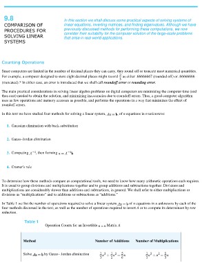
In Table 1 we list the number of operations required to solve a linear system of n equations in n unknowns by each of the

four methods discussed in the text, as well as the number of operations required to invert A or to compute its determinant by row

reduction.

Table 1 Matrix A

Operation Counts for an Invertible

Method Number of Additions Number of Multiplications

Solve by Gauss– Jordan elimination