Page 79 - Hall et al (2015) Principles of Critical Care-McGraw-Hill

CHAPTER 7: Interpreting and Applying Evidence in Critical Care Medicine 47

differences in outcomes between groups reflect true differences or sim- skill in the correct interpretation of diagnostic tests. To correctly inter-
ply chance variation, also known as random error. pret a variety of diagnostic tests, one must understand how well that test
At the conceptual level, there are four possible results of any given study: reflects the actual presence or absence of disease in any given patient.
The sensitivity and specificity of a given test reflect how closely the result
1. There is an observed difference in outcomes between two groups, of that test reflects the truth about a patient’s disease process.
which represents a true association between the predictor and the The sensitivity of a test is the proportion of people with the disease in
outcome. question that will have a positive test result. A highly sensitive test will
2. There is no observed difference in outcomes between two groups, identify the majority of patients who actually have that disease and will
which correctly represents a true lack of association between the yield very few false-negative results. The specificity of a test measures the
predictor and the outcome. proportion of people without the disease that have a negative test. A highly
3. There is an observed difference in outcomes between two groups when specific test will identify the majority of those who do not have the dis-
https://kat.cr/user/tahir99/
there is no true association between the predictor and the outcome. ease and will have very few false-positive results. In order to evaluate the
4. There is no observed difference in outcomes between two groups, sensitivity and specificity of a new diagnostic test, it must be tested against
another highly reliable method of identifying the disease, referred to as the
when, in fact, there is an association between the predictor and the “gold standard.” Sensitivity and specificity are best visualized, understood,
outcome. 20 and calculated using a 2 × 2 table, as shown in the example below:
A Type I error is exemplified by number three above, in which the
investigator has incorrectly concluded that there is a difference between A biotech company markets their “PE-Dx,” a bedside, noninvasive
two groups when there is no true difference. The p value is a measure diagnostic test for pulmonary embolism (PE), as a scientific
of the probability that this type of error occurred. Significance testing breakthrough. Your institution studies 2000 patients using PE-Dx.
compares study findings with the “null hypothesis,” which states that
there is no difference between the groups in question. Many incorrectly Those patients also undergo pulmonary angiogram, the gold standard
interpret the p value as the probability that there is truly no difference test for PE. A total of 800 patients have a PE diagnosed via angiogram,
between the groups (ie, the null hypothesis is true), given the results of of whom 400 have a positive PE-Dx. Among those with a negative
the study. The p value, however, is correctly interpreted as the prob-
21
ability of obtaining the given study results or something more extreme angiogram, 300 have a positive PE-Dx.
if there is truly no difference between the groups. By convention, a p
21
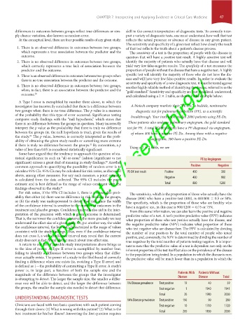
value of less than 0.05 is considered statistically significant. Using a 2 × 2 table, we see
Some have argued that the tendency to approach the question of sta-
tistical significance in such an “all-or-none” fashion (significant vs not PE by Angiogram
significant) misses a great deal of meaning in study findings. Another
22
common approach to quantifying the possibility of random error is to Positive Negative
calculate 95% CIs. 95% CIs may be calculated for risk ratios, as discussed PE-DX test result Positive 400 300
above, among other measures. For any such measure, a point estimate
is calculated from the data collected. The 95% CI includes the point Negative 400 900
estimate and is best defined as the range of values consistent with the Total 800 1200
findings observed in the study. 21
For risk ratios, if the 95% CI includes 1, there is a reasonable prob- The sensitivity, which is the proportion of those who actually have the
ability that either (a) there was no difference in risk between the groups, disease (800) who have a positive test (400), is 400/800 = 0.5 or 50%.
or (b) the study was underpowered to detect that risk, since the width The specificity, which is the proportion of those who are healthy who
of the confidence interval is sensitive to the number of outcomes in the have a negative test, in this case is 900/1200 = 0.75 or 75%.
treatment and placebo groups. Confidence intervals also aid in the inter- From this same information, we can also learn the positive and negative
pretation of the precision with which a given outcome is determined. predictive value of a test. A test’s positive predictive value (PPV) indicates
That is, the narrower the confidence interval, the more precisely we may what proportion of those who test positive actually have the disease, and
understand the effect size of a given study. Or, put another way, the wider the negative predictive value (NPV) indicates what proportion of those
the confidence interval, the less well characterized is the range of values who test negative who are disease free. The PPV is calculated by dividing
consistent with the study findings. Thus, even if the confidence interval the number of true positives by the total number of people who tested
does not cross 1, a wide confidence interval may reveal that the current positive, and, conversely, the NPV is determined by dividing the number of
study does not in fact reveal all that much about true effect size. true negatives by the total number of patients testing negative. It is impor-
A return to our list of possible study interpretations above brings us tant to note that the predictive value of a test is dependent not only on the
to the idea of power. A Type II error is exemplified by number four, inherent properties of the test itself but also on the prevalence of the disease
failing to identify a difference between two groups when that differ- in the population being tested. In a population in which the disease is rare,
ence actually exists. The power of a study is the likelihood of correctly the predictive value will be much lower than in a population in which the
finding a difference when one exists (ie, avoiding a Type II error) and
is defined as 1—the probability of committing a Type II error. A study’s
power is, in large part, a function of both the sample size and the
magnitude of the difference between the groups that the investigator Patients With Patients Without
is attempting to detect. The larger the sample size, the smaller a differ- Disease Disease Total
ence one will be able to detect, and the larger the difference between 1% Disease prevalence Test positive 19 40 59
the groups, the smaller the sample size needed to detect that difference. Test negative 1 1940 1941
Total 20 1980 2000
UNDERSTANDING DIAGNOSTIC TESTS
10% Disease prevalence Test positive 190 90 280
Clinicians are faced with two basic questions with each patient coming Test negative 10 1710 1720
through their doors: (1) What is wrong with this patient? (2) What is the
best treatment for his/her illness? Answering the first question requires Total 200 1800 2000

Section01.indd 47 1/22/2015 9:36:58 AM