Page 51 - The Atlas of Economic Complexity

52 | THE ATLAS OF ECONOMIC COMPLEXITY

t e c h n I c a l B o x 5 . 1 : m e a s u r I n g p r o x I m I t y

to make products you need chunks of embedded knowledge which we call stringent. For instance, in the year 2008, 17 countries exported wine, 24 ex-
capabilities. the capabilities needed to produce one good may or may not be ported grapes and 11 exported both, all with rCa>1. then, the proximity between
useful in the production of other goods. since we do not observe capabilities wines and grapes is 11/24=0.46. note that we divide by 24 instead of 17 to mini-
directly, we create a measure that infers the similarity between the capabili- mize false positives. Formally, for a pair of goods and we define proximity as:
ties required by a pair of goods by looking at the probability that they are co-
exported. to quantify this similarity we assume that if two goods share most
of the requisite capabilities, the countries that export one will also export the
other. By the same token, goods that do not share many capabilities are less
likely to be co-exported.
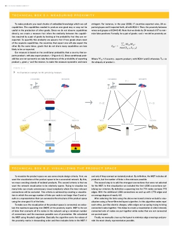
our measure is based on the conditional probability that a country that ex-
ports product will also export product (Figure 5.1.1). since conditional prob-
abilities are not symmetric we take the minimum of the probability of exporting Where =1 if country exports product with rCa>1 and 0 otherwise. is
product , given and the reverse, to make the measure symmetric and more the ubiquity of product .

FIGURE 5.1.1:
An illustrative example for the proximity measure.

X-RAY MACHINES MEDICAMENTS X-RAY MACHINES MEDICAMENTS
P = 1

NETHERLANDS (NLD)
P = 1/2 P = 1/3

CHEESE CREAMS AND POLISHES FROZEN FISH CHEESE FROZEN FISH
CREAMS AND POLISHES

ARGENTINA (ARG) GHANA (GHA)

t e c h n I c a l B o x 5 . 2 : v I s u a l I z I n g t h e p r o d u c t s pa c e

to visualize the product space we use some simple design criteria. First, we and only if they connect an isolated product. By definition, the Mst includes all
want the visualization of the product space to be a connected network. By this, products, but the number of links is the minimum possible.
we mean avoiding islands of isolated products. the second criteria is that we the second step is to add the strongest connections that were not selected
want the network visualization to be relatively sparse. trying to visualize too for the Mst. in this visualization we included the first 1,006 connections sat-
many links can create unnecessary visual complexity where the most relevant isfying our criterion. By definition a spanning tree for 774 nodes contains 773
connections will be occluded. this criteria is achieved by creating a visualiza- edges. With the additional 1,006 connections we end up with 1,779 edges and
tion in which the average number of links per node is not larger than 5 and re- an average degree of nearly 4.6.
sults in a representation that can summarize the structure of the product space after selecting the links using the above mentioned criteria we build a visu-
using the strongest 1% of the links. alization using a Force-Directed layout algorithm. in this algorithm nodes repel
to make sure the visualization of the product space is connected, we calcu- each other, just like electric charges, while edges act as spring trying to bring
late the maximum spanning tree (Mst) of the proximity matrix. Mst is the set connected nodes together. this helps to create a visualization in which densely
of links that connects all the nodes in the network using a minimum number connected sets of nodes are put together while nodes that are not connected
of connections and the maximum possible sum of proximities. We calculated are pushed apart.
the Mst using Kruskal’s algorithm. Basically the algorithm sorts the values of Finally, we manually clean up the layout to minimize edge crossings and pro-
the proximity matrix in descending order and then includes links in the Mst if vide the most clearly representation possible.