Page 274 - Jolliffe I. Principal Component Analysis

241
10.1. Detection of Outliers Using Principal Components
outliers is proposed by Gabriel and Zamir (1979). This proposal uses the
idea of weighted PCs, and will be discussed further in Section 14.2.1.
Projection pursuit was introduced in Section 9.2.2 as a family of tech-
niques for finding clusters, but it can equally well be used to look for
outliers. PCA is not specifically designed to find dimensions which best
display either clusters or outliers. As with clusters, optimizing a criterion
other than variance can give better low-dimensional displays in which to
identify outliers. As noted in Section 9.2.2, projection pursuit techniques
find directions in p-dimensional space that optimize some index of ‘interest-
ingness,’ where ‘uninteresting’ corresponds to multivariate normality and
‘interesting’ implies some sort of ‘structure,’ such as clusters or outliers.
Some indices are good at finding clusters, whereas others are better at
detecting outliers (see Friedman (1987); Huber (1985); Jones and Sibson
(1987)). Sometimes the superiority in finding outliers has been observed
empirically; in other cases the criterion to be optimized has been chosen
with outlier detection specifically in mind. For example, if outliers rather
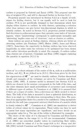
than clusters are of interest, Caussinus and Ruiz (1990) suggest replacing
the quantity in equation (9.2.1) by

∗ 2

∗
∗
n K[ x i − x S −1](x i − x )(x i − x )
ˆ
Γ = i=1 2 , (10.1.5)
n ∗
i=1 K[ x i − x S −1]
where x is a robust estimate of the centre of the x i such as a multivariate
∗
median, and K[.], S are defined as in (9.2.1). Directions given by the first
−1
ˆ
few eigenvectors of SΓ are used to identify outliers. Further theoretical
details and examples of the technique are given by Caussinus and Ruiz-
Gazen (1993, 1995). A mixture model is assumed (see Section 9.2.3) in
which one element in the mixture corresponds to the bulk of the data, and
the other elements have small probabilities of occurrence and correspond
to different types of outliers. In Caussinus et al. (2001) it is assumed that
if there are q types of outlier, then q directions are likely needed to detect
them. The bulk of the data is assumed to have a spherical distribution, so
there is no single (q+1)th direction corresponding to these data. The ques-
tion of an appropriate choice for q needs to be considered. Using asymptotic
results for the null (one-component mixture) distribution of a matrix which
ˆ
is closely related to SΓ −1 , Caussinus et al. (2001) use simulation to derive
tables of critical values for its eigenvalues. These tables can then be used
to assess how many eigenvalues are ‘significant,’ and hence decide on an
appropriate value for q. The use of the tables is illustrated by examples.
The choice of the value of β is discussed by Caussinus and Ruiz-Gazen
(1995) and values in the range 0.1to0.5 are recommended. Caussinus
et al. (2001) use somewhat smaller values in constructing their tables,
which are valid for values of β in the range 0.01 to 0.1. Penny and Jol-
liffe (2001) include Caussinus and Ruiz-Gazen’s technique in a comparative