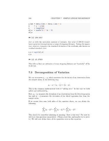
Page 104 - Applied Statistics with R

104 CHAPTER 7. SIMPLE LINEAR REGRESSION

y_hat = beta_0_hat + beta_1_hat * x
e = y - y_hat
n = length(e)
s2_e = sum(e^2) / (n - 2)
s2_e

## [1] 236.5317

Just as with the univariate measure of variance, this value of 236.53 doesn’t
have a practical interpretation in terms of stopping distance. Taking the square
root, however, computes the standard deviation of the residuals, also known as
residual standard error.

s_e = sqrt(s2_e)
s_e

## [1] 15.37959

This tells us that our estimates of mean stopping distance are “typically” off by
15.38 feet.

7.3 Decomposition of Variation

We can re-express − ̄, which measures the deviation of an observation from

the sample mean, in the following way,

− ̄ = ( − ̂ ) + ( ̂ − ̄).

This is the common mathematical trick of “adding zero.” In this case we both

added and subtracted ̂ .

Here, − ̂ measures the deviation of an observation from the fitted regression

̂
line and − ̄ measures the deviation of the fitted regression line from the

sample mean.
If we square then sum both sides of the equation above, we can obtain the
following,

2
2
2
∑( − ̄ ) = ∑( − ̂ ) + ∑( ̂ − ̄ ) .

=1 =1 =1
This should be somewhat alarming or amazing. How is this true? For now we
will leave this questions unanswered. (Think about this, and maybe try to prove
it.) We will now define three of the quantities seen in this equation.