Page 100 - Applied Statistics with R

100 CHAPTER 7. SIMPLE LINEAR REGRESSION

̂
̂
̂ = + .
0
1
In this case,
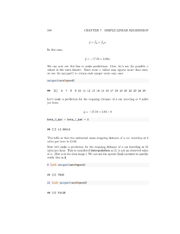
̂ = −17.58 + 3.93 .

We can now use this line to make predictions. First, let’s see the possible
values in the cars dataset. Since some values may appear more than once,
we use the unique() to return each unique value only once.

unique(cars$speed)

## [1] 4 7 8 9 10 11 12 13 14 15 16 17 18 19 20 22 23 24 25

Let’s make a prediction for the stopping distance of a car traveling at 8 miles
per hour.

̂ = −17.58 + 3.93 × 8

beta_0_hat + beta_1_hat * 8

## [1] 13.88018

This tells us that the estimated mean stopping distance of a car traveling at 8
miles per hour is 13.88.

Now let’s make a prediction for the stopping distance of a car traveling at 21
miles per hour. This is considered interpolation as 21 is not an observed value
of . (But is in the data range.) We can use the special %in% operator to quickly
verify this in R.

8 %in% unique(cars$speed)

## [1] TRUE

21 %in% unique(cars$speed)

## [1] FALSE