Page 99 - Applied Statistics with R

7.2. LEAST SQUARES APPROACH 99

x = cars$speed
y = cars$dist

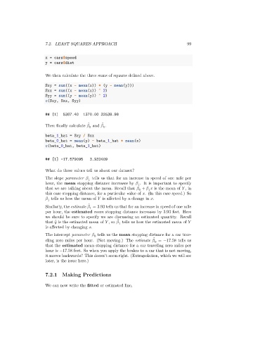
We then calculate the three sums of squares defined above.
Sxy = sum((x - mean(x)) * (y - mean(y)))
Sxx = sum((x - mean(x)) ^ 2)
Syy = sum((y - mean(y)) ^ 2)
c(Sxy, Sxx, Syy)

## [1] 5387.40 1370.00 32538.98

̂
̂
Then finally calculate and .
1
0
beta_1_hat = Sxy / Sxx
beta_0_hat = mean(y) - beta_1_hat * mean(x)
c(beta_0_hat, beta_1_hat)

## [1] -17.579095 3.932409

What do these values tell us about our dataset?

The slope parameter tells us that for an increase in speed of one mile per
1
hour, the mean stopping distance increases by . It is important to specify
1
that we are talking about the mean. Recall that + is the mean of , in
0
1
this case stopping distance, for a particular value of . (In this case speed.) So
tells us how the mean of is affected by a change in .
1
̂
Similarly, the estimate = 3.93 tells us that for an increase in speed of one mile
1
per hour, the estimated mean stopping distance increases by 3.93 feet. Here
we should be sure to specify we are discussing an estimated quantity. Recall
̂
that ̂ is the estimated mean of , so tells us how the estimated mean of

1
is affected by changing .
The intercept parameter tells us the mean stopping distance for a car trav-
0
̂
eling zero miles per hour. (Not moving.) The estimate = −17.58 tells us
0
that the estimated mean stopping distance for a car traveling zero miles per
hour is −17.58 feet. So when you apply the brakes to a car that is not moving,
it moves backwards? This doesn’t seem right. (Extrapolation, which we will see
later, is the issue here.)
7.2.1 Making Predictions
We can now write the fitted or estimated line,