Page 210 - Applied Statistics with R

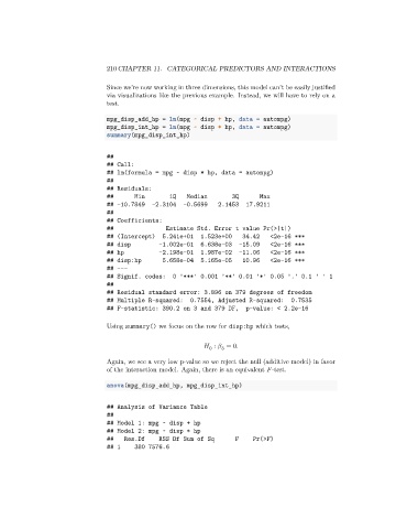
210 CHAPTER 11. CATEGORICAL PREDICTORS AND INTERACTIONS

Since we’re now working in three dimensions, this model can’t be easily justified
via visualizations like the previous example. Instead, we will have to rely on a
test.

mpg_disp_add_hp = lm(mpg ~ disp + hp, data = autompg)
mpg_disp_int_hp = lm(mpg ~ disp * hp, data = autompg)
summary(mpg_disp_int_hp)

##
## Call:
## lm(formula = mpg ~ disp * hp, data = autompg)
##
## Residuals:
## Min 1Q Median 3Q Max
## -10.7849 -2.3104 -0.5699 2.1453 17.9211
##
## Coefficients:
## Estimate Std. Error t value Pr(>|t|)
## (Intercept) 5.241e+01 1.523e+00 34.42 <2e-16 ***
## disp -1.002e-01 6.638e-03 -15.09 <2e-16 ***
## hp -2.198e-01 1.987e-02 -11.06 <2e-16 ***
## disp:hp 5.658e-04 5.165e-05 10.96 <2e-16 ***
## ---
## Signif. codes: 0 '***' 0.001 '**' 0.01 '*' 0.05 '.' 0.1 ' ' 1
##
## Residual standard error: 3.896 on 379 degrees of freedom
## Multiple R-squared: 0.7554, Adjusted R-squared: 0.7535
## F-statistic: 390.2 on 3 and 379 DF, p-value: < 2.2e-16

Using summary() we focus on the row for disp:hp which tests,

∶ = 0.
0
3
Again, we see a very low p-value so we reject the null (additive model) in favor
of the interaction model. Again, there is an equivalent -test.

anova(mpg_disp_add_hp, mpg_disp_int_hp)

## Analysis of Variance Table
##
## Model 1: mpg ~ disp + hp
## Model 2: mpg ~ disp * hp
## Res.Df RSS Df Sum of Sq F Pr(>F)
## 1 380 7576.6