Page 234 - Applied Statistics with R

234 CHAPTER 12. ANALYSIS OF VARIANCE

## 19 3.571440 control
## 20 9.784136 treatment

Here, we would like to test,

∶ = vs ∶ ≠

1

0
To do so in R, we use the t.test() function, with the var.equal argument set
to TRUE.
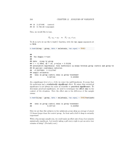
t.test(sleep ~ group, data = melatonin, var.equal = TRUE)

##
## Two Sample t-test
##
## data: sleep by group
## t = -2.0854, df = 18, p-value = 0.05154
## alternative hypothesis: true difference in means between group control and group treatment is not equal to 0
## 95 percent confidence interval:
## -3.02378261 0.01117547
## sample estimates:
## mean in group control mean in group treatment
## 6.827152 8.333456

At a significance level of = 0.10, we reject the null hypothesis. It seems that
the melatonin had a statistically significant effect. Be aware that statistical
significance is not always the same as scientific or practical significance. To
determine practical significance, we need to investigate the effect size in the
context of the situation. Here the effect size is the difference of the sample
means.

t.test(sleep ~ group, data = melatonin, var.equal = TRUE)$estimate

## mean in group control mean in group treatment
## 6.827152 8.333456

Here we see that the subjects in the melatonin group sleep an average of about
1.5 hours longer than the control group. An hour and a half of sleep is certainly
important!
With a big enough sample size, we could make an effect size of say, four minutes
statistically significant. Is it worth taking a pill every night to get an extra four
minutes of sleep? (Probably not.)