Page 237 - Applied Statistics with R

12.3. ONE-WAY ANOVA 237

• is the overall sample mean.
̄
2
• is the sample variance of group .

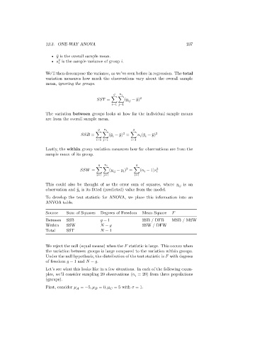
We’ll then decompose the variance, as we’ve seen before in regression. The total
variation measures how much the observations vary about the overall sample
mean, ignoring the groups.

= ∑ ∑( − ̄) 2

=1 =1
The variation between groups looks at how far the individual sample means
are from the overall sample mean.

2

= ∑ ∑( ̄ − ̄) = ∑ ( ̄ − ̄) 2

=1 =1 =1
Lastly, the within group variation measures how far observations are from the
sample mean of its group.

2
= ∑ ∑( − ̄ ) = ∑( − 1) 2

=1 =1 =1
This could also be thought of as the error sum of squares, where is an

observation and ̄ is its fitted (predicted) value from the model.

To develop the test statistic for ANOVA, we place this information into an
ANVOA table.
Source Sum of Squares Degrees of Freedom Mean Square
Between SSB − 1 SSB / DFB MSB / MSW
Within SSW − SSW / DFW
Total SST − 1

We reject the null (equal means) when the statistic is large. This occurs when
the variation between groups is large compared to the variation within groups.
Under the null hypothesis, the distribution of the test statistic is with degrees
of freedom − 1 and − .
Let’s see what this looks like in a few situations. In each of the following exam-
ples, we’ll consider sampling 20 observations ( = 20) from three populations

(groups).
First, consider = −5, = 0, = 5 with = 1.