Page 283 - Applied Statistics with R

13.3. UNUSUAL OBSERVATIONS 283

points(x = point_3[1], y = point_3[2], pch = 1, cex = 4, col = "black", lwd = 2)
abline(ex_model, col = "dodgerblue", lwd = 2)
abline(model_3, lty = 2, col = "darkorange", lwd = 2)
legend("bottomleft", c("Original Data", "Added Point"),
lty = c(1, 2), col = c("dodgerblue", "darkorange"))

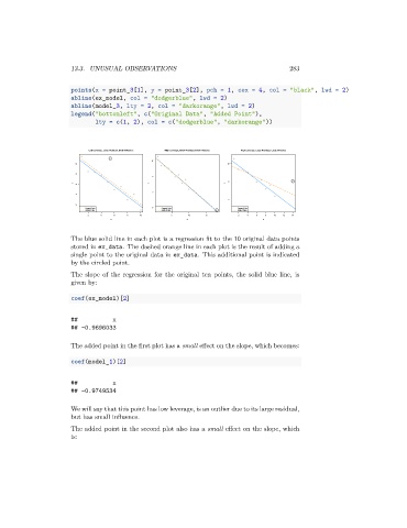
Low Leverage, Large Residual, Small Influence High Leverage, Small Residual, Small Influence High Leverage, Large Residual, Large Influence
10
10 10
8
5
5
y 6 y y
0
4
0
2
Original Data -5 Original Data Original Data
Added Point Added Point Added Point
2 4 6 8 10 5 10 15 2 4 6 8 10 12 14
x x x
The blue solid line in each plot is a regression fit to the 10 original data points
stored in ex_data. The dashed orange line in each plot is the result of adding a
single point to the original data in ex_data. This additional point is indicated
by the circled point.
The slope of the regression for the original ten points, the solid blue line, is
given by:

coef(ex_model)[2]

## x
## -0.9696033

The added point in the first plot has a small effect on the slope, which becomes:

coef(model_1)[2]

## x
## -0.9749534

We will say that this point has low leverage, is an outlier due to its large residual,
but has small influence.
The added point in the second plot also has a small effect on the slope, which
is: