Page 286 - Applied Statistics with R

286 CHAPTER 13. MODEL DIAGNOSTICS

lev_ex = data.frame(
x1 = c(0, 11, 11, 7, 4, 10, 5, 8),
x2 = c(1, 5, 4, 3, 1, 4, 4, 2),
y = c(11, 15, 13, 14, 0, 19, 16, 8))

plot(x2 ~ x1, data = lev_ex, cex = 2)
points(7, 3, pch = 20, col = "red", cex = 2)

5

4

x2 3

2

1
0 2 4 6 8 10

x1

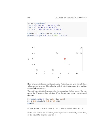
Here we’ve created some multivariate data. Notice that we have plotted the
values, not the values. The red point is (7, 3) which is the mean of x1 and the
mean of x2 respectively.
We could calculate the leverages using the expressions defined above. We first
create the matrix, then calculate as defined, and extract the diagonal
elements.

X = cbind(rep(1, 8), lev_ex$x1, lev_ex$x2)
H = X %*% solve(t(X) %*% X) %*% t(X)
diag(H)

## [1] 0.6000 0.3750 0.2875 0.1250 0.4000 0.2125 0.5875 0.4125

Notice here, we have two predictors, so the regression would have 3 parameters,
so the sum of the diagonal elements is 3.