Page 352 - Applied Statistics with R

352 CHAPTER 14. TRANSFORMATIONS

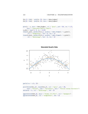
fit_2 = lm(y ~ poly(x, 2), data = data_higher)
fit_4 = lm(y ~ poly(x, 4), data = data_higher)

plot(y ~ x, data = data_higher, col = "grey", pch = 20, cex = 1.5,
main = "Simulated Quartic Data")
x_plot = seq(-5, 5, by = 0.05)
lines(x_plot, predict(fit_2, newdata = data.frame(x = x_plot)),
col = "dodgerblue", lwd = 2, lty = 1)
lines(x_plot, predict(fit_4, newdata = data.frame(x = x_plot)),
col = "darkorange", lwd = 2, lty = 2)

Simulated Quartic Data

10

5

0
y
-5

-10

-2 -1 0 1 2
x

par(mfrow = c(1, 2))

plot(fitted(fit_2), resid(fit_2), col = "grey", pch = 20,
xlab = "Fitted", ylab = "Residuals", main = "Fitted versus Residuals")
abline(h = 0, col = "darkorange", lwd = 2)

qqnorm(resid(fit_2), main = "Normal Q-Q Plot", col = "darkgrey")
qqline(resid(fit_2), col = "dodgerblue", lwd = 2)