Page 353 - Applied Statistics with R

14.2. PREDICTOR TRANSFORMATION 353

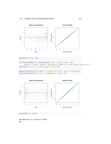
Fitted versus Residuals Normal Q-Q Plot

5 5
Residuals 0 Sample Quantiles 0

-5 -5

-8 -6 -4 -2 0 -3 -2 -1 0 1 2 3
Fitted Theoretical Quantiles

par(mfrow = c(1, 2))

plot(fitted(fit_4), resid(fit_4), col = "grey", pch = 20,
xlab = "Fitted", ylab = "Residuals", main = "Fitted versus Residuals")
abline(h = 0, col = "darkorange", lwd = 2)

qqnorm(resid(fit_4), main = "Normal Q-Q Plot", col = "darkgrey")
qqline(resid(fit_4), col = "dodgerblue", lwd = 2)

Fitted versus Residuals Normal Q-Q Plot

5 5

Residuals 0 Sample Quantiles 0

-5 -5

-6 -4 -2 0 2 -3 -2 -1 0 1 2 3
Fitted Theoretical Quantiles

anova(fit_2, fit_4)

## Analysis of Variance Table
##