Page 445 - Applied Statistics with R

17.4. CLASSIFICATION 445

17.4.2 Evaluating Classifiers

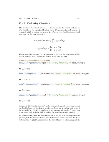
The metric we’ll be most interested in for evaluating the overall performance
of a classifier is the misclassification rate. (Sometimes, instead accuracy is
reported, which is instead the proportion of correction classifications, so both
metrics serve the same purpose.)

̂
̂
Misclass( , Data) = 1 ∑ ( ≠ (x ))
i
=1
̂

i
̂
( ≠ (x )) = { 0 = (x )
i

̂
1 ≠ (x )
i

When using this metric on the training data, it will have the same issues as RSS
did for ordinary linear regression, that is, it will only go down.
# training misclassification rate
mean(ifelse(predict(fit_caps) > 0, "spam", "nonspam") != spam_trn$type)
## [1] 0.339

mean(ifelse(predict(fit_selected) > 0, "spam", "nonspam") != spam_trn$type)

## [1] 0.224

mean(ifelse(predict(fit_additive) > 0, "spam", "nonspam") != spam_trn$type)

## [1] 0.066

mean(ifelse(predict(fit_over) > 0, "spam", "nonspam") != spam_trn$type)

## [1] 0.136

Because of this, training data isn’t useful for evaluating, as it would suggest that
we should always use the largest possible model, when in reality, that model is
likely overfitting. Recall, a model that is too complex will overfit. A model that
is too simple will underfit. (We’re looking for something in the middle.)
To overcome this, we’ll use cross-validation as we did with ordinary linear re-
gression, but this time we’ll cross-validate the misclassification rate. To do so,
we’ll use the cv.glm() function from the boot library. It takes arguments for