Page 440 - Applied Statistics with R

440 CHAPTER 17. LOGISTIC REGRESSION

## ---
## Signif. codes: 0 '***' 0.001 '**' 0.01 '*' 0.05 '.' 0.1 ' ' 1
##
## (Dispersion parameter for binomial family taken to be 1)
##
## Null deviance: 596.11 on 461 degrees of freedom
## Residual deviance: 477.45 on 454 degrees of freedom
## AIC: 493.45
##
## Number of Fisher Scoring iterations: 5

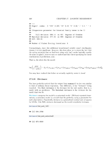
Unsurprisingly, since this additional transformed variable wasn’t intelligently
chosen, it is not significant. However, this does allow us to stress the fact that
the syntax notation that we had been using with lm() works basically exactly
the same for glm(), however now we understand that this is specifying the linear
combination of predictions, (x).

That is, the above fits the model

(x)
log ( ) = + + + + + + + 2
3 famhist
4 typea
2 ldl
0
1 alcohol
7 ldl
6 ldl famhist
5 age
1 − (x)
You may have realized this before we actually explicitly wrote it down!
17.3.8 Deviance
You have probably noticed that the output from summary() is also very similar
to that of ordinary linear regression. One difference, is the “deviance” being
reported. The Null deviance is the deviance for the null model, that is, a
model with no predictors. The Residual deviance is the deviance for the
model that was fit.
Deviance compares the model to a saturated model. (Without repeated obser-
vations, a saturated model is a model that fits perfectly, using a parameter for
each observation.) Essentially, deviance is a generalized residual sum of squares
for GLMs. Like RSS, deviance decreased as the model complexity increases.
deviance(chd_mod_ldl)

## [1] 564.2788

deviance(chd_mod_selected)

## [1] 475.6856