Page 394 - Color_Atlas_of_Physiology_5th_Ed._-_A._Despopoulos_2003

The exponents of the multiplicands are Graphic Representation of Data
added together when multiplying powers of
10, and the denominator is subtracted from the Graphic plots of data are used to provide a
numerator when dividing powers of ten. clear and concise representation of measure-
Examples: ments, e.g., body temperature over the time of
3
2
10 · 10 = 10 2+ 3 = 10 5 day (! C). The axes on which the measure-
4
2
10 % 10 = 10 4 - 2 = 10 2 ments (e.g., temperature and time) are plotted
10 % 10 = 10 2 - 4 = 10 -2 are called coordinates. The vertical axis is re-
2
4
The usual mathematical rules apply to the ferred to as the ordinate (temperature) and the
multipliers of powers of ten, e.g., horizontal axis is the abscissa (time). It is cus-
3
(3 · 10 · (2 · 10 ) = (2 · 3) · (10 2+ 3 ) = 6 · 10 . 5 tomary to plot the first variable x (time) on the
2
Logarithms. There are two kinds of loga- abscissa and the other dependent variable y
rithms: common and natural. Logarithmic cal- (temperature) on the ordinate. The abscissa is
culations are performed using exponents therefore called the x-axis and the ordinate the Logarithms, Graphic Representation of Data
alone. The common (decimal) logarithm (log y-axis. This method of graphically plotting data
or lg) is the power or exponent to which 10 can be used to illustrate the connection be-
must be raised to equal the number in ques- tween any two related dimensions imaginable,
tion. The common logarithm of 100 (log 100) is e.g., to describe the relationship between
2, for example, because 10 = 100. Decimal height and age, lung capacity and intrapulmo-
2
logarithms are commonly used in physiology, nary pressure, etc. (! p. 117).
e.g., to define pH values (see above) and to plot Plotting of data makes it easier to determine
the pressure of sound on a decibel scale whether two variables correlate with each
(! p. 363). other. For example, the plot of height (ordi-
Natural logarithms (ln) have a natural base nate) over age (abscissa) shows that the height
of 2.71828..., also called base e. The common increases during the growth years and reaches
logarithm (log x) equals the natural logarithm a plateau at the age of about 17 years. This
of x (ln x) divided by the natural logarithm of means that height is related to age in the first
10 (ln 10), where ln 10 = 2.302585. The follow- phase of life, but is largely independent of age
ing rules apply when converting between nat- in the second phase. A correlation does not
ural and common logarithms: necessarily indicate a causal relationship. A
log x = (ln x)/2.3 decrease in the birth rate in Alsace-Lorraine,
ln x = 2.3 · log x. for example, correlated with a decrease in the
When performing mathematical operations number or nesting storks for a while.
with logarithms, the type of operation is re- When plotting variables of wide-ranging di-
duced by one rank—multiplication becomes mensions (e.g., 1 to 100 000) on a coordinate
addition, potentiation becomes multiplica-
tion, and so on.
Examples:
log (a · b) = log a + log b 37.5
log (a/b) = log a - log b °C
n
log a = n · log a
n
log !"a = (log a)/n Body temperature (rectal, at rest) 37.0
Special cases:
log 10 = ln e = 1
log 1 = ln 1 = 0 36.5
12
6
12
12
6
log 0 = ln 0 = & ' p.m. p.m. a.m. a.m. p.m.
Time of day
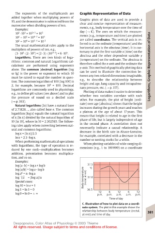
C. Illustration of how to plot data on a coordi-
nate system. The plot in this example shows the
relationship between body temperature (rectal, 381
at rest) and time of day.
Despopoulos, Color Atlas of Physiology © 2003 Thieme
All rights reserved. Usage subject to terms and conditions of license.