Page 396 - Color_Atlas_of_Physiology_5th_Ed._-_A._Despopoulos_2003

y = ax + b, many enzyme reactions and carrier-mediated
where a is the slope of the line and b is the transport processes:
point, or intercept (at x = 0), where it intersects C
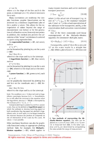
the y-axis. J = J max · K M + C [13.10]
Many correlations are nonlinear. For sim- where J is the actual rate of transport (e.g., in
pler functions, graphic linearization can be mol · m · s ), J max is the maximal transport
–1
–2
achieved via a nonlinear (logarithmic) plot of rate, C (mol · m ) is the actual concentration of
–3
the x and/or y values. This allows for the ex- the substance to be transported, and K M is the
trapolation of values beyond the range of concentration (half-saturation concentration)
measurement (see below) or for the genera- at /2 J max.
1
tion of calibration curves from only two points. One of the three commonly used linear
In addition, this method also permits the cal- rearrangements of the Michaelis–Menten
culation of the “mean” correlation of scattered equation, the Lineweaver–Burk plot, states:
x-y pairs using regression lines.
An exponential function (! D1, red curve), 1/J = (K M/J max) · (1/C) + 1/J max, [13.11]
such as Consequently, a plot of 1/J on the y-axis and
y = a · e b · x , 1/C on the x-axis results in a straight line Graphic Representation of Data
can be linearized by plotting ln y on the y-axis (! E2). While a plot of J over C (! E1) does not
(! D2):
ln y = ln a + b · x,
where b is the slope and ln a is the intercept.
A logarithmic function (! D1, blue curve), 1
such as J J max
y = a + b · ln x,
can be linearized by plotting ln x on the x-axis
(! D4), where b is the slope and a is the inter- J = J max ·C/(K M +C)
cept. 1 / 2 J max
A power function (! D1, green curve), such
as
y = a · x , b
can be graphically linearized by plotting ln y
and ln x on the coordinate axes (! D3) be- 0 C
cause
K M
ln y = ln a + b · ln x,
where b is the slope and ln a is the intercept. 2 1/J
Note: The condition x or y = 0 does not exist on loga-
rithmic coordinates because ln 0 = '. Nevertheless,
ln a is still called the intercept in the equation when
the logarithmic abscissa (! D3,4) is intercepted by
the ordinate at ln x = 0, i.e., x = 1.
Instead of plotting ln x and/or ln y on the x- and/or
y-axis, they can be plotted on logarithmic paper on 1/J max Range of
which the ordinate or abscissa (semi-log paper) or measurement
both coordinates (log-log paper) are plotted in loga-
rithmic units. In such cases, a is no longer treated as 0 1/C
the intersect because the position of a depends on –1/K M
site of intersection of the x-axis by the y-axis. All E. Two methods of representing the Mi-
values ( 0 are possible. chaelis–Menten equation: The data can be
Other nonlinear functions can also be graphi- plotted as a curve of J over C (E1), or as 1/J over
cally linearized using an appropriate plotting 1/C in linearized form (E2). In the latter case,
method. Take, for example, the Michaelis– Jmax and K M are determined by extrapolating 383
the data outside the range of measurement.
Menten equation (! E1), which applies to
Despopoulos, Color Atlas of Physiology © 2003 Thieme
All rights reserved. Usage subject to terms and conditions of license.