
Page 29 - TCS ICT Book 7
P. 29
The City School 2021-2022
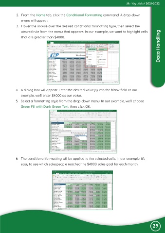
2. From the Home tab, click the Conditional Formatting command. A drop-down
menu will appear.
3. Hover the mouse over the desired conditional formatting type, then select the
desired rule from the menu that appears. In our example, we want to highlight cells
Data Handling
that are greater than $4000.
4. A dialog box will appear. Enter the desired value(s) into the blank field. In our
example, we’ll enter $4000 as our value.
5. Select a formatting style from the drop-down menu. In our example, we’ll choose
Green Fill with Dark Green Text, then click OK.
6. The conditional formatting will be applied to the selected cells. In our example, it’s
easy to see which salespeople reached the $4000 sales goal for each month.
29