Page 147 - Robot Design Handbook ROBOCON Malaysia 2019

function which is from the library of opencv. After that, the BRG image is converted into

HSV by using ‘cvtColor’ function. HSV is further converted into binary image by ‘inRange’
function. The line will become white colour, everything other than the line will become

black [4]. After that, an auto calibration will be carried out where the robot will auto
calibrate the image until it sees there is only a straight white line in the binary image. Auto

calibration is carried by using ‘inRange’, ‘HoughLines’ transform and ‘findContours’. The

parameter for inRange function is the HSV value.

inRange( frame_HSV, Scalar(low_H, low_S,
low_V),Scalar(high_H, high_S, high_V),frame_threshold);

Our programme will continuously manipulate the parameter for the HSV value
boundary until it detects there is only one contour from ‘findContours’ and two lines from

‘HoughLines’. Function ‘findContours’ can detect how many contours are there in the
image. Function ‘HoughLines’ transform can detect how many straight lines are there in the

image. For example, if the robot wants to differentiate between yellow and white colour.

The initial parameter for ‘inRange’ function will be like this.

inRange(frame_HSV, Scalar(low_H, 0, 0), Scalar(180, 255,
255), frame_threshold);

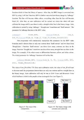
The value of low_H will be 179. Once auto-calibration starts, the value of low_H will start

to decrease until the programme detects there are only one contour and two straight lines in

the binary image. Auto-calibration will only be run at Gobi Urtuu and Mountain Urtuu
which had been circled in the purple-colour rectangular box (see Figure 3).

Figure 9: The map of the Figure 10: The binary image with
competition. contours and centroids.

143