Page 136 - Applied Statistics with R

136 CHAPTER 8. INFERENCE FOR SIMPLE LINEAR REGRESSION

We write,

∼
to say that the random variable follows a distribution with degrees of
freedom.
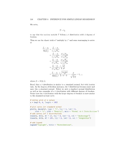
Then we use the classic trick of “multiply by 1” and some rearranging to arrive
at

̂
̂
− 1 = − 1
1
1
̂
SE[ ] /√

1
̂
− 1 /√
1
= ⋅
/√ /√

̂
− /√
= 1 1 ⋅
/√ /√

̂
− 1 2
1
= / √
/√ 2
̂
− ( −2) 2
2
= 1 1 / √ ∼ ∼ −2
̂
SD[ ] − 2 √ 2 −2
1
−2
where ∼ (0, 1).
Recall that a distribution is similar to a standard normal, but with heavier
tails. As the degrees of freedom increases, the distribution becomes more and
more like a standard normal. Below we plot a standard normal distribution
as well as two examples of a distribution with different degrees of freedom.
Notice how the distribution with the larger degrees of freedom is more similar
to the standard normal curve.
# define grid of x values
x = seq(-4, 4, length = 100)
# plot curve for standard normal
plot(x, dnorm(x), type = "l", lty = 1, lwd = 2,
xlab = "x", ylab = "Density", main = "Normal vs t Distributions")
# add curves for t distributions
lines(x, dt(x, df = 1), lty = 3, lwd = 2, col = "darkorange")
lines(x, dt(x, df = 10), lty = 2, lwd = 2, col = "dodgerblue")

# add legend
legend("topright", title = "Distributions",