Page 133 - Applied Statistics with R

8.2. SAMPLING DISTRIBUTIONS 133

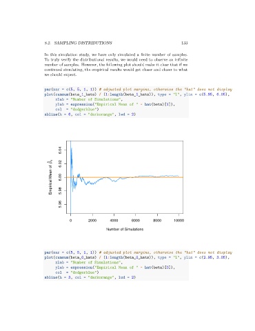
In this simulation study, we have only simulated a finite number of samples.
To truly verify the distributional results, we would need to observe an infinite
number of samples. However, the following plot should make it clear that if we
continued simulating, the empirical results would get closer and closer to what
we should expect.

par(mar = c(5, 5, 1, 1)) # adjusted plot margins, otherwise the "hat" does not display
plot(cumsum(beta_1_hats) / (1:length(beta_1_hats)), type = "l", ylim = c(5.95, 6.05),
xlab = "Number of Simulations",
ylab = expression("Empirical Mean of " ~ hat(beta)[1]),
col = "dodgerblue")
abline(h = 6, col = "darkorange", lwd = 2)

6.04

Empirical Mean of β 1 6.00 5.98
^ 6.02

5.96

0 2000 4000 6000 8000 10000
Number of Simulations

par(mar = c(5, 5, 1, 1)) # adjusted plot margins, otherwise the "hat" does not display
plot(cumsum(beta_0_hats) / (1:length(beta_0_hats)), type = "l", ylim = c(2.95, 3.05),
xlab = "Number of Simulations",
ylab = expression("Empirical Mean of " ~ hat(beta)[0]),
col = "dodgerblue")
abline(h = 3, col = "darkorange", lwd = 2)