Page 135 - Applied Statistics with R

8.3. STANDARD ERRORS 135

̂
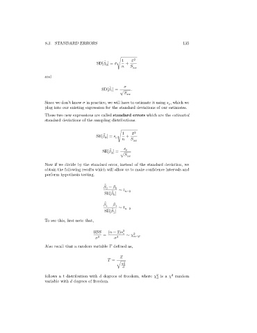
SD[ ] = √ 1 + 2 ̄
0

and

̂
SD[ ] = .
1
√
Since we don’t know in practice, we will have to estimate it using , which we

plug into our existing expression for the standard deviations of our estimates.
These two new expressions are called standard errors which are the estimated
standard deviations of the sampling distributions.

̂
SE[ ] = √ 1 + 2 ̄
0

̂
SE[ ] =
1
√
Now if we divide by the standard error, instead of the standard deviation, we
obtain the following results which will allow us to make confidence intervals and
perform hypothesis testing.

̂
− 0 ∼
0
̂
SE[ ] −2
0
̂
− 1 ∼
1
̂
SE[ ] −2
1
To see this, first note that,
RSS ( − 2) 2 2
2 = 2 ∼ −2 .

Also recall that a random variable defined as,

=
√ 2

2
2
follows a distribution with degrees of freedom, where is a random

variable with degrees of freedom.