Page 131 - Applied Statistics with R

8.2. SAMPLING DISTRIBUTIONS 131

beta_1 # true mean

## [1] 6

var(beta_1_hats) # empirical variance

## [1] 0.11899

var_beta_1_hat # true variance

## [1] 0.1176238

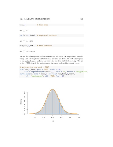
We see that the empirical and true means and variances are very similar. We also
verify that the empirical distribution is normal. To do so, we plot a histogram
̂
of the beta_1_hats, and add the curve for the true distribution of . We use
1
prob = TRUE to put the histogram on the same scale as the normal curve.
# note need to use prob = TRUE
hist(beta_1_hats, prob = TRUE, breaks = 20,
xlab = expression(hat(beta)[1]), main = "", border = "dodgerblue")
curve(dnorm(x, mean = beta_1, sd = sqrt(var_beta_1_hat)),
col = "darkorange", add = TRUE, lwd = 3)

1.0
0.8

Density 0.6

0.4

0.2

0.0

5.0 5.5 6.0 6.5 7.0 7.5
^
β 1