Page 139 - Applied Statistics with R

8.6. CARS EXAMPLE 139

8.6 cars Example

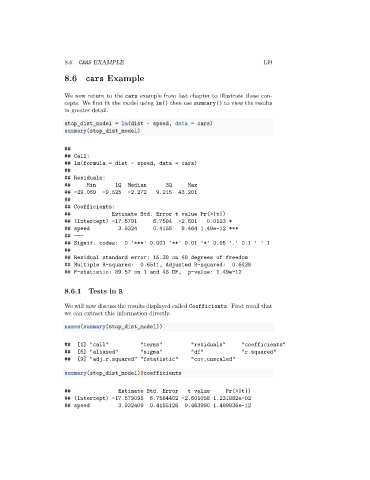
We now return to the cars example from last chapter to illustrate these con-
cepts. We first fit the model using lm() then use summary() to view the results
in greater detail.

stop_dist_model = lm(dist ~ speed, data = cars)
summary(stop_dist_model)

##
## Call:
## lm(formula = dist ~ speed, data = cars)
##
## Residuals:
## Min 1Q Median 3Q Max
## -29.069 -9.525 -2.272 9.215 43.201
##
## Coefficients:
## Estimate Std. Error t value Pr(>|t|)
## (Intercept) -17.5791 6.7584 -2.601 0.0123 *
## speed 3.9324 0.4155 9.464 1.49e-12 ***
## ---
## Signif. codes: 0 '***' 0.001 '**' 0.01 '*' 0.05 '.' 0.1 ' ' 1
##
## Residual standard error: 15.38 on 48 degrees of freedom
## Multiple R-squared: 0.6511, Adjusted R-squared: 0.6438
## F-statistic: 89.57 on 1 and 48 DF, p-value: 1.49e-12

8.6.1 Tests in R

We will now discuss the results displayed called Coefficients. First recall that
we can extract this information directly.

names(summary(stop_dist_model))

## [1] "call" "terms" "residuals" "coefficients"
## [5] "aliased" "sigma" "df" "r.squared"
## [9] "adj.r.squared" "fstatistic" "cov.unscaled"

summary(stop_dist_model)$coefficients

## Estimate Std. Error t value Pr(>|t|)
## (Intercept) -17.579095 6.7584402 -2.601058 1.231882e-02
## speed 3.932409 0.4155128 9.463990 1.489836e-12